Our approach has been to treat spatial and temporal correlation in data as a nuisance, problems to be addressed after we've fit the best model we can using the predictors at our disposal. Beginning in lecture 15 we examined data in which measurements were obtained over time on the same subject as well as on different subjects yielding a hierarchical data structure with the potential for residual temporal correlation. Beginning in lecture 30 we turned to spatially referenced data where even after fitting a regression model with spatially referenced predictors the spatial correlation persisted. Today we examine a data set in which the residuals of our best regression model exhibit both temporal and spatial correlation.
To illustrate this we return to a data set that was analyzed in Assignment 8. The data consist of repeated observations over a four year period on 691 different parcels of land in eastern North Carolina. The goal was to determine factors that affect the decision to use burning as a land management tool. We used GEE to fit a logistic regression model to the binary response. GEE provides marginal interpretations of the parameters rather than the subject-specific interpretations provided by mixed effects models, and was needed to deal with the unusual temporal correlation structure exhibited by the data. Observations separated by three years were positively correlated while observations separated by one or two years were negatively correlated. This correlation structure is consistent with the rule-of-thumb that recommends burning every three years.
I load the data and fit a GEE model with an unstructured correlation matrix. For completeness I fit the model using both the gee and geepack packages.
The data consist of repeated observations on parcels of land. Because the parcels are spatially referenced and have spatial extent there is the potential for spatial correlation. For instance, it's not unreasonable for nearby parcels to have been burned at the same. As a first step toward understanding this we plot the physical locations of the parcels and examine their distance relationships.
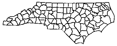
To help display the spatial relationships between parcels I obtain a state and county boundary shapefile from the North Carolina Geodetic Survey web site. Shapefiles can be read into R with functions from the maptools package. Below I use the readShapePoly function for this purpose.
Fig. 1 Plot of North Carolina shapefile
Because the coordinates of each site appear multiple times in the data set (for each of the four years of measurement), I use the tapply function to extract one set of coordinates from each site.
To zoom in on the portion of North Carolina where the data are, I use the ranges of the plot coordinates to set the x-limits and y-limits of the North Carolina shapefile map. We're told that the map is scaled in feet, while the coordinates in the burn data set are scaled in meters, so we need to use a meters-to-feet conversion factor when plotting the sites. I also subtract and add a small amount to the lower and upper limits of the range when specifying the limits in the plot function.
I also add a key showing the distance scale used on the map.
 |
|
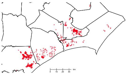
| Fig. 2 Spatial distribution of parcels (PolyFIDs) from the burn data set in North Carolina |
The map reveals a substantial amount of clustering of the parcels. Unlike the wheat yield data we examined in lecture 32 where the observations were equally spaced, the spatial distribution of the burn sites is quite patchy consisting of both dense and loose clusters of points some with large gaps between them. To get a better sense of the distances involved I calculate all the pairwise distances between sites and examine their distribution.
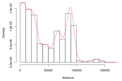
So sites are as close as 22 meters and as far as part as 165 kilometers! I display a histogram of the distances and superimpose a kernel density estimate using the density function. Because the boundary value of zero will distort the kernel density estimate, I append to the distances their negative values and fit the kernel density to both. I then discard the negative values and double the remaining y-coordinates so that the area under the kernel density still integrates to 1. I begin by converting the "dist" object created by the dist function to a matrix and extract the unique distances that lie in the lower triangle of the matrix. The distribution of distances turns out to be distinctly bimodal with a long tail.
 |
|
| Fig. 3 Histogram and kernel density estimate of the distribution of inter-parcel distances |
We next turn to assessing whether there is lingering spatial correlation in the residuals from the GEE model. Because the Mantel and semivariogram functions require that all the observations have distinct coordinates so that none of the pairwise distances are zero, I restrict the analysis to just the residuals from 2004. I extract the spatial coordinates and Pearson residuals from the geeglm model and subset them by year.
I use the mantel function from vegan to obtain a randomization test of the Mantel correlation of the residual distances in 2004 with the geographic distances.
Call:
mantel(xdis = dist.g, ydis = dist.r)
Mantel statistic r: 0.05939
Significance: 0.001
Empirical upper confidence limits of r:
90% 95% 97.5% 99%
0.0171 0.0230 0.0307 0.0397
Based on 999 permutations
The correlation although small is statistically significant. As we'll see the small correlation is probably due to the very local nature of the spatial correlation coupled with the very large spatial extent of the data. Only nearby observations are correlated; the vast majority of the observations are uncorrelated.
So how do we account for the spatial correlation in a way that will also allows us to simultaneously account for the temporal correlation? In lecture 32 we had success by including the spatial coordinates of the observations as predictors in the model, either in the form of a response surface or as nonparametric smoothers in a GAM. Using this approach here we would just need to add appropriate geographic terms to the regression equation in the GEE model for temporal correlation. Unfortunately this approach doesn't work here. Adding geographic terms to the mean process model does not substantially reduce the spatial correlation. This shouldn't be surprising because it's unlikely that the large-scale geographic location of a site has much to do with the decision to burn or not. Such decisions are likely to be very local affecting only whether adjacent sites are burned together or not, a decision that does not vary with latitude and longitude. Contrast this with the effect of geography on wheat yield in the experiment of lecture 32. There unmeasured soil conditions that varied geographically could easily have led to the spatial correlation in yield that was detected.
Because the parcels have areal extent we could view these as lattice data and define neighborhoods for each parcel consisting of those parcels that share boundaries with a given parcel. A frequently used spatial correlation model for lattice data is the ICAR model, an acronym for the intrinsic conditional autoregressive model. In a CAR model each parcel is assigned its own unique random effect but also receives the weighted inputs from the random effects of its neighbors. This is a kind of mixed effects model but because of its complicated nature it is most easily implemented using Bayesian methods. Because we need to couple the spatial correlation with a temporal correlation that we saw in Assignment 8 was not correctly captured by including random effects, we can reject a CAR model for these data.
Given that GEE was able to effectively handle the temporal correlation it would be nice if we could add the spatial correlation to the GEE model. When the data are sorted by parcel and there is only temporal correlation among observations from the same parcel, the correlation matrix of the full data set is a block diagonal matrix in which the temporal correlation matrix occurs repeatedly along the diagonal, once for each parcel, and there are zeros everywhere else. A straightforward way to extend a temporal correlation matrix to a spatio-temporal correlation matrix is to make the additional assumption that the space-time covariance is separable, meaning that it can be written as the product of a spatial covariance and a temporal covariance. See, e.g., Gumpertz et al. (2000) and Lin (2010).
With the assumption of separability the spatio-temporal correlation matrix is obtained as the Kronecker product of the spatial correlation matrix estimated from a variogram, say, and the temporal correlation matrix estimated from GEE or directly from the model residuals. In the Kronecker product the temporal correlations appear repeatedly as identical 4 × 4 matrices along the block diagonal. These same blocks also appear in the off-diagonal positions but multiplied by an appropriate spatial decay constant that decreases as a function of the distance separating the plots. These off-diagonal elements describe how the temporal correlation pattern for observations from the same site is diminished by spatial extent when observations from different sites are considered. The main attraction of separability apart from its simplicity is that if the temporal matrix and the spatial matrix are both legitimate correlation matrices (i.e., they are both invertible and positive definite), then the Kronecker product of these two matrices will also be a legitimate correlation matrix. There is no guarantee of this happening when the matrix is assembled in a piecemeal fashion.
As an illustration suppose A is a 2 × 2 spatial correlation matrix and B is a 3 × 3 temporal correlation matrix.
Then the Kronecker product, ![]() is defined to be the following 6 × 6 matrix.
is defined to be the following 6 × 6 matrix.
For the burn data set we would choose A to be a 691 × 691 matrix of spatial correlations between the 691 parcels and B to be the 4 × 4 matrix of temporal correlations among the four years 2004 through 2007. The final matrix ![]() is 2764 × 2764, the dimensionality of the data set.
is 2764 × 2764, the dimensionality of the data set.
We can construct the spatial correlation matrix A and/or the complete spatio-temporal correlation matrix C in a number of ways. I list three.
In all cases it is necessary to check the entries of the constructed spatio-temporal correlation matrix for feasibility. The Prentice bounds for binary data must still hold and the functions presented in lecture 23 can be used to check this. Given the way in which the correlation matrix was constructed, feasibility violations in the spatial part of the matrix should be corrected by adjusting the parameters of the overall semivariogram model that was used to generate the matrix, rather than by tweaking only the individual matrix entries that violate the bounds.
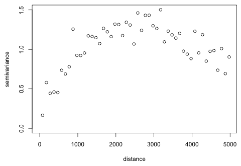
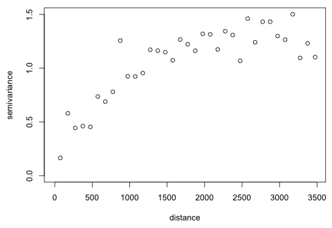
I use the 2004 residuals to estimate a semivariogram model. I start by generating the empirical semivariogram. I try bins with centers that are a distance 100 m apart and extend the calculations out to 5000 meters.
The first bin clearly has too few observations so I try moving the center of the first bin to a larger value.
 |
|
| Fig. 4 Semivariogram of 2004 residuals from a GEE model |
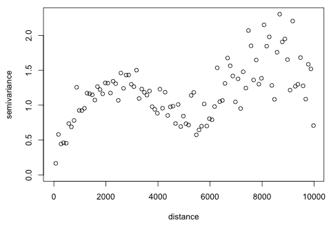
The graph seems to be turning back on itself after reaching what appears to be a sill of around 1.3. I try extending the graph out even further to see if this pattern persists.
 |
|
| Fig. 5 Semivariogram of 2004 residuals from a GEE model carried out to 10,000 meters. |
Now we see that at around 3000 m the graph becomes quite noisy and begins to oscillate around the putative sill of 1.3. Considering the arrangement of parcels shown in Fig. 2 the patchiness of the data set may be causing this. Once a certain distance is reached the semivariances are being calculated between observations from clusters that are geographically disjoint. The mean process model probably doesn't adequately account for all the spatial heterogeneity in the data set and this is manifesting itself in the noisy semivariogram at greater distances. In any case it's pretty clear that the local correlation that we're trying to detect dissipates at around 3500 m, so we should stop calculating the semivariances at that point. We'll fit theoretical models to this semivariogram in the next lecture.
 |
|
| Fig. 6 Semivariogram of 2004 residuals from a GEE model |
| Jack Weiss Phone: (919) 962-5930 E-Mail: jack_weiss@unc.edu Address: Curriculum for the Environment and Ecology, Box 3275, University of North Carolina, Chapel Hill, 27599 Copyright © 2012 Last Revised--April 3, 2012 URL: https://sakai.unc.edu/access/content/group/2842013b-58f5-4453-aa8d-3e01bacbfc3d/public/Ecol562_Spring2012/docs/lectures/lecture33.htm |