Assignment 8—Solution

Question 1

Model: binomial, link: logit

Response: burn50

Terms added sequentially (first to last)

                         Df Deviance Resid. Df Resid. Dev Pr(>Chi)   
NULL                                      2763       2321            
Hectares                  1      8.4      2762       2312   0.0037 **
factor(rx_cat3)           3    107.7      2759       2205  < 2e-16 ***
zmin_drd                  1     23.1      2758       2181  1.5e-06 ***
prop_timb                 1      8.2      2757       2173   0.0042 **
Prop_no_b                 1     31.7      2756       2142  1.8e-08 ***
zmin_dr                   1     32.0      2755       2110  1.5e-08 ***
zmin_ddv                  1      2.8      2754       2107   0.0961 . 
factor(rx_cat3):zmin_ddv  3     25.4      2751       2081  1.3e-05 ***
---
Signif. codes:  0 ‘***’ 0.001 ‘**’ 0.01 ‘*’ 0.05 ‘.’ 0.1 ‘ ’ 1

Question 2

Question 3

I obtain the QIC, CIC, sum of the absolute differences between the naive parameter standard errors and the robust parameter standard errors, and the sum of the absolute differences of the naive parameter covariance matrix and the robust parameter covariance matrix. I assemble the results in a matrix and identify the winners.

The independence model has the smallest QIC, the unstructured model has the smallest CIC, the exchangeable model has the lowest sum of absolute standard error differences, and the unstructured model has the lowest sum of absolute covariance differences. The proponents of CIC note that for models that do not predict the mean well, QIC does a poor job of selecting the correct correlation structure, while CIC performs better. Given that the unstructured matrix is the winner using CIC and one additional metric, at this point I would lean toward using the unstructured correlation matrix.

Question 4

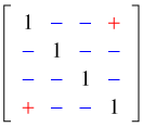
The data span the years 2004 through 2007. A manager who followed the rule of thumb and who burned in 2004 would then not burn in 2005, not burn in 2006, but burn again in 2007. Thus response variable in 2004 is negatively correlated with the response variable in 2005 and 2006, but positively correlated with it in 2007. Thus in the four year span, observations that are one or two years apart should be negatively correlated while observations that are three years apart should be positively correlated. The correlation matrix would be expected to contain terms whose signs exhibit the following pattern.

If we examine the estimated unstructured correlation matrix it is exactly of this form with all negative values on the off-diagonal except in the (1, 4) position, which is positive.

Question 5

Question 6

The fact that the GLM and GLMM solutions are identical suggests that the GLMM has converged to the GLM solution, i.e., a model without random effects. We can verify this by examining the log-likelihoods of these two models as well as the variance components of the mixed effects model. The log-likelihoods are identical and the variance component is essentially zero.

attr(,"sc")
[1] NA

When this happens it means the model has converged to a local solution rather than the global solution. Under normal circumstances we might try to reparameterize the model or fiddle with control settings, but those are unlikely to be successful here. A random intercepts model induces an exchangeable correlation structure within clusters so that all members of the group are equally correlated to each other and positively so. We've already seen from Question 4 that this is probably the wrong correlation structure for these data. Consequently a random intercepts model is probably the wrong model for these data too.

Question 7

I create a matrix in which all the possible pairs of the four different years appear as row entries.

I next use the Prentice function from class to calculate upper and lower bounds for the six entries in the correlation matrix corresponding to these pairs of years.

The entries in the (1,3) and (2,3) positions exceed the Prentice bounds. The estimated values are far too negative.

Question 8

I replace the entries in the (1,3) and (2,3) positions with –0.11 and –0.05 respectively (as well as the corresponding entries in the lower triangle).

Question 9

The geepack package requires that we extract the lower triangle of the correlation matrix we wish to use and then replicate it with the rep function as many times as there are different groups in the data set. The number of groups is the number of unique values of the plot indicator PolyFID.

To fit the model with geeglm I enter this as the zcor argument and specify corst="fixed".

 Coefficients:
                           Estimate   Std.err   Wald Pr(>|W|)   
(Intercept)               -1.697391  0.138567 150.05  < 2e-16 ***
Hectares                   0.000698  0.000325   4.61   0.0317 * 
factor(rx_cat3)2           0.669453  0.162977  16.87  4.0e-05 ***
factor(rx_cat3)3           0.537899  0.260912   4.25   0.0392 * 
factor(rx_cat3)4           0.250123  0.215030   1.35   0.2447   
zmin_drd                   0.056454  0.025438   4.93   0.0265 * 
prop_timb                 -0.752567  0.277991   7.33   0.0068 **
Prop_no_b                 -0.982047  0.233089  17.75  2.5e-05 ***
zmin_dr                   -0.460432  0.107152  18.46  1.7e-05 ***
zmin_ddv                   0.026709  0.076397   0.12   0.7266   
factor(rx_cat3)2:zmin_ddv -0.200711  0.129358   2.41   0.1208   
factor(rx_cat3)3:zmin_ddv  1.093507  0.343279  10.15   0.0014 **
factor(rx_cat3)4:zmin_ddv  0.179461  0.089204   4.05   0.0442 * 
---
Signif. codes:  0 ‘***’ 0.001 ‘**’ 0.01 ‘*’ 0.05 ‘.’ 0.1 ‘ ’ 1

Scale is fixed.

Correlation: Structure = fixed  Link = identity

Estimated Correlation Parameters:
        Estimate Std.err
alpha:1        1       0
Number of clusters:   691   Maximum cluster size: 4

It turns out this model could also have been fit using the gee function of the gee package. We need to use corst="fixed" with the R= argument in which we specify the correlation matrix for the largest sized group. As usual the group is identifed with the id variable.

Model:
 Link:                      Logit
 Variance to Mean Relation: Binomial
 Correlation Structure:     Fixed

Call:
gee(formula = burn50 ~ Hectares + factor(rx_cat3) + zmin_drd +
    prop_timb + Prop_no_b + zmin_dr + zmin_ddv + zmin_ddv:factor(rx_cat3),
    id = PolyFID, data = burn, R = new.mat, family = binomial,
    corstr = "fixed", scale.fix = T)

Summary of Residuals:
    Min      1Q  Median      3Q     Max
-0.6635 -0.1880 -0.1085 -0.0221  0.9921

Coefficients:
                           Estimate Naive S.E. Naive z Robust S.E. Robust z
(Intercept)               -1.697391   0.165405 -10.262    0.138567   -12.25
Hectares                   0.000698   0.000317   2.203    0.000325     2.15
factor(rx_cat3)2           0.669453   0.179328   3.733    0.162977     4.11
factor(rx_cat3)3           0.537899   0.265638   2.025    0.260912     2.06
factor(rx_cat3)4           0.250123   0.221797   1.128    0.215030     1.16
zmin_drd                   0.056454   0.031749   1.778    0.025438     2.22
prop_timb                 -0.752567   0.293341  -2.565    0.277991    -2.71
Prop_no_b                 -0.982047   0.209656  -4.684    0.233089    -4.21
zmin_dr                   -0.460432   0.091942  -5.008    0.107152    -4.30
zmin_ddv                   0.026709   0.087260   0.306    0.076397     0.35
factor(rx_cat3)2:zmin_ddv -0.200711   0.121673  -1.650    0.129358    -1.55
factor(rx_cat3)3:zmin_ddv  1.093507   0.348452   3.138    0.343279     3.19
factor(rx_cat3)4:zmin_ddv  0.179461   0.098064   1.830    0.089204     2.01

Estimated Scale Parameter:  1
Number of Iterations:  4

Working Correlation
       [,1]   [,2]    [,3]    [,4]
[1,]  1.000 -0.160 -0.1100  0.2462
[2,] -0.160  1.000 -0.0500 -0.1632
[3,] -0.110 -0.050  1.0000 -0.0857
[4,]  0.246 -0.163 -0.0857  1.0000

Course Home Page