As appealing as mixed effects models are for handling hierarchical clustered/correlated data, the difficulties (discussed last time) in interpreting the parameter estimates from generalized linear mixed effects models with non-identity links suggests that other approaches are needed. One of the most popular of these is generalized estimating equations (GEE). GEE extends generalized linear models to correlated data but differs from mixed effects models in that GEE explicitly fits a marginal model to data. To understand the motivation behind GEE we need to take a closer look at the theory behind generalized linear models.
The probability distributions used in generalized linear models are related because they are all members of what's called the exponential family of distributions. The density (mass) function of any member of the exponential family takes the following form.
|
(1) |
|---|
The functions a, b, and c in the formula will vary from distribution to distribution. The parameter θ is called the canonical parameter and is a function of μ. This function of μ is referred to as the canonical link function.
Example: As an illustration we write the Poisson distribution in its exponential form. The formula for the Poisson probability mass function is shown below.

Through a series of steps we can transform this expression into one that is of the correct exponential form.

Comparing this to the generic exponential form

we can make the following identifications.
* * * * *
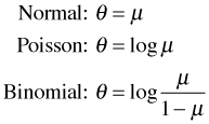
The canonical link functions for three members of the exponential family of probability distributions are shown below.

These in turn are the usual link functions used in normal, Poisson, and logistic regression. The mean and variance of a distribution in the exponential family are given generically as follows.

The last step defines Var(μ) as the derivative of the mean with respect to the canonical parameter.
Suppose we have a random sample of size n from a member of the exponential family of distributions. The likelihood is given by

with corresponding log-likelihood
 .
.
To find maximum likelihood estimates analytically we take the derivative of the log-likelihood with respect to the canonical parameter θ, set the result equal to zero, and solve for θ.

Typically we do this in a regression setting in which we express the canonical parameter as a linear combination of predictors.

So, in this case we would differentiate the log-likelihood with respect to each of the regression parameters separately, set the result equal to zero, and solve for the regression parameters. The shorthand notation for this is to use a vector derivative (gradient).

After some algebraic simplification and using the notation defined previously, we end up with p + 1 equations of the following form.
|
(2) |
|---|
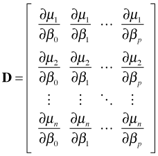
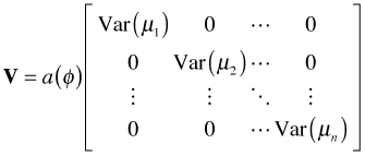
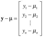
These are referred to as estimating equations because we can use them to obtain the maximum likelihood estimate of β. The p + 1 estimating equations defined by eqn (2) can be written more succinctly using matrix notation. Define the n × (p + 1) matrix D, the n × n matrix V, and the n × 1 vector y – μ as follows.
 , , |
 , , |

With these definitions the p + 1 estimating equations of eqn (2) can be written as the following single matrix equation.
|
(3) |
|---|
The primary problem in dealing with correlated data in a likelihood framework is that the likelihood becomes inordinately complicated. Generalized estimating equations gets around this difficulty by making the following simple observation. Although the likelihood in eqn (1) depends specifically on the form of the probability distribution, (the functions a, b, and c), the estimating equation that we obtain by differentiating the log-likelihood that is shown in eqns (2) and (3) depends on the probability distribution only via the mean μ and the variance V. The rest of the details about the nature of the original probability distribution are irrelevant. So, when a probability model is a member of the exponential family we don't need the all the details of the probability distribution in order to estimate the parameters of a regression equation, just its mean and variance.
Inspired by this observation, generalized estimating equations performs an end-around the likelihood. Rather than starting with eqn (1), GEE starts with the estimating equations in eqn (2), or equivalently the matrix version eqn (3), and generalizes it in two distinct ways.
![]()
where S is a diagonal matrix and R is the proposed correlation matrix for our data. Typically R will depend on parameters that need to be estimated from the data when solving eqn (3). If so, an additional estimating equation will be required.
Both of these two generalizations lead to what is called a generalized estimating equation. Parameter estimates are obtained by solving the generalized estimating equations numerically typically using an optimization algorithm based on Newton's method.
The estimating equation of eqn (1) is the derivative of the log-likelihood set equal to zero.

From calculus we know that the process of differentiation can be reversed by integrating (antidifferentiating) this expression. Because we can add an arbitrary constant to an antiderivative and obtain another antiderivative, antidifferentiation does not yield a unique result. Antidifferentiating the estimating equation yields the following.

If we start with this last integral, there are two possible scenarios.
|
(4) |
|---|
The connection between quasi-likelihood and likelihood theory is actually quite close. It turns out that GEE estimates have the same large sample properties that MLEs do—they're consistent, asymptotically normal, etc. In addition, the quasi-likelihood can be used to generate an AIC-like quantity for use in model selection.
When estimating a regression model using maximum likelihood (for instance fitting a generalized linear model) we
When fitting a model using generalized estimating equations we
In most GEE software the mean-variance relationship is identified by specifying, using a family argument, a probability model that has the same mean-variance relationship as the one desired. This convention is rather counterintuitive given that there is no probability model in GEE. Table 1 lists some typical choices for the family argument in GEE and the corresponding expression for Var(μ) that results from that choice.
Table 1 Common mean-variance relationships in GEE
| Var(μ) | Family |
1 |
gaussian (normal) |
μ |
poisson |
μ(1 – μ) |
binomial (Bernoulli) |
μ2 |
gamma |
Depending on the software, a scale parameter φ can also be estimated to account for over- or under-dispersion in Poisson and binomial models.
Table 2 defines some of the common correlation models that are available in GEE software. (The exact name used will depend on the software.) The correlation requested in GEE is referred to as the working correlation and for 2-level hierarchical data it refers to the correlation among observations j and k coming from the same level-2 unit i.
Table 2 Common correlation structures in GEE
| Correlation type | Correlation formula |
| independence | |
| exchangeable | |
| AR(1) | |
| unstructured | |
| user-defined | Specific values are entered for the correlations |
Typically there is also an ID argument that is used to identify the variable that denotes the level-2 units. This is the same as the group variable in mixed effects models. (In nlme the group variable appeared to the right of the vertical bar in the random argument: random = ~1|group_variable.)
The family argument of the glm function of R permits the use of quasibinomial, quasipoisson, or the more general quasi function. These are not probability distributions per se but are ways to specify a model for Var(μ) in the manner described in Table 1 above. The quasipoisson and quasibinomial choices generalize the expressions given in Table 1 as follows.
Table 3 The quasi values for the family argument
| Family | Var(μ) |
| quasipoisson | φμ |
| quasibinomial | φμ(1 – μ) |
Here  is called the dispersion parameter. The Pearson deviance is the sum of the squared Pearson residuals. The quasi function can be used to specify these same variance structures as well as others by giving a formula for the variance along with a link function. For instance, family=quasi(var="mu(1-mu)", link=logit) yields the same result as family=quasibinomial.
The quasipoisson and quasibinomial families provide a crude way to adjust for overdispersion in data, where overdispersion is defined as deviation from the Poisson or binomial probability models due to clumping. When either family = quasipoisson or family = quasibinomial is specified, the parameter estimates one gets from glm are identical to what one gets with family = poisson or family = binomial, but the standard errors are adjusted by multiplying them by the square root of φ.
Full-fledged GEE, on the other hand, assumes the data have a hierarchical structure in which the clusters are identified explicitly with an ID variable. GEE also allows you to model the correlation in a cluster by using one of the correlation structures of Table 2.
There are three recommended methods for choosing a correlation structure for GEE (Hardin & Hilbe, 2003).
I examine the last two options in more detail.
QIC is due to Pan (2001) and comes in two flavors. One version is used for selecting a correlation structure and the second version is used for choosing models all of which were fit with the same correlation structure. I first discuss the version of QIC that is used for choosing a correlation structure.
In what follows let R denote the correlation structure of interest and let I denote the independence model. Recall the definition of AIC.
![]()
QIC is defined analogously as follows.
|
(5) |
|---|
The first term contains the quasi-likelihood as given in eqn (4) except that it is now extended to the full data set.

The quasi-likelihood defined in this formula is actually a bit of a hybrid. For ![]() we use the regression coefficient estimates obtained from a GEE model with correlation model R, but for Var(μ) we assume a working correlation structure of independence I. Table 4 gives the quasi-likelihood formulas (multiplied by φ) for models in which the mean-variance relationship has the form of a binomial or a Poisson random variable.
we use the regression coefficient estimates obtained from a GEE model with correlation model R, but for Var(μ) we assume a working correlation structure of independence I. Table 4 gives the quasi-likelihood formulas (multiplied by φ) for models in which the mean-variance relationship has the form of a binomial or a Poisson random variable.
Table 4 Quasi-likelihoods
| Family | Var(μ) | |
| binomial | μ(1 – μ) |  |
| Poisson | μ |  |
For binary data (binomial with n = 1) the estimate of φ described above is not used; instead φ is set to one. The second term of QIC, ![]() , is a penalty term that is analogous to 2K in the formula for AIC. It is defined as follows.
, is a penalty term that is analogous to 2K in the formula for AIC. It is defined as follows.
So, to calculate QIC we need to fit two models: one that uses the correlation model R and the other that uses the independence model I. QIC is then used like AIC. We make various choices for R and choose the R that yields the lowest value of QIC.
Pan (2001) also suggested another version of QIC for comparing models that have the same working correlation matrix R and the same quasi-likelihood form (for instance, all Poisson), but involve different predictor sets. He suggested calculating a statistic QICu that is defined as follows.
![]()
Models with smaller values of QICu are to be preferred.
Recently QIC has been criticized as a model selection tool, particularly if the model for the mean does not fit the data very well. Hin and Wang (2009) argue that the two terms in the expression for QIC in eqn (5) are not equally informative for correctly identifying the correlation structure. In particular the quasi-likelihood term corresponds to an apparent error rate that better indicates an inadequacy in the mean model rather than in the correlation model. Through simulations they demonstrate that when the mean model is misspecified, the quasi-likelihood term can mask differences in model quality that are due purely to the different assumptions made about the correlation. As a result they recommend using just the second term of QIC (without the superfluous multiplier of two) when comparing models with different correlation structures. They call this statistic the correlation information criterion, CIC.
![]()
All GEE packages return something that is variously referred to as the sandwich variance estimate or the robust variance estimate. For many packages this is the default estimate that is displayed in the standard error column of the summary table of the model. The sandwich estimate corrects the variance estimate that is based on the working correlation matrix R using a correction that is constructed from the model residuals. It tends to be robust to an incorrectly specified working correlation model R and will be nearly correct even if R is incorrect. The sandwich estimate is known to behave best for a large sample consisting of many small groups so that there are not too many observations in each group. If the total number of groups is small, the sandwich estimate can be very biased.
In addition to the sandwich variance estimate, GEE packages also return a variance estimate that is based only on the working correlation model R. This is variously called the model-based variance estimate or the naive variance estimate.
A correlation model R can be selected as follows. Fit a series of models that differ only in the choice of correlation matrix R; all of the remaining features of these models are the same. For each model compare the sandwich variance estimates with the model-based variance estimates. The model whose sandwich variance estimates most closely resembles its model-based variance estimates is the one with the best correlation model R.
In addition to invertibility and positive definiteness, correlation matrices for binary data have a further feasibility requirement (Chaganty and Joe 2004). The predicted probabilities of a pair of binary response variables impose a constraint on the legal values that the correlation can take. Let yi and yj be two binary observations, let pi and pj be their predicted probabilities under a given model, and let rij be their correlation as estimated from say a GEE model. Prentice (1998) derived the following formula for the joint probability of the binary pair yi and yj.

Because probabilities must be non-negative, the expression inside the brackets imposes a constraint on the possible values the correlation rij can take.
Currently available GEE software, including the gee and geepack packages of R, do not check for the feasibility of the correlation matrices they estimate for binary data. The general consensus is that if a correlation estimated by GEE is infeasible that is a good reason to reject that correlation model. There has been a lot of discussion of this issue in the biomedical and biostatistical literature. For a recent survey see Ziegler and Vens (2010) as well as the discussion that follows the article (Breitung et al. 2010; Shults 2011).
| Jack Weiss Phone: (919) 962-5930 E-Mail: jack_weiss@unc.edu Address: Curriculum for the Environment and Ecology, Box 3275, University of North Carolina, Chapel Hill, 27599 Copyright © 2012 Last Revised--February 29, 2012 URL: https://sakai.unc.edu/access/content/group/2842013b-58f5-4453-aa8d-3e01bacbfc3d/public/Ecol562_Spring2012/docs/lectures/lecture22.htm |