Lecture 21—Monday, February 27, 2012

Topics

• Correlated data analysis III: Generalized estimating equations (GEE)
• Variable transformations versus link functions
  • Transforming the response variable
  • Choosing a probability distribution and a link function
• Marginal and subject-specific interpretations of a mixed effects model
  • Identity link
  • Logit link
    • Subject-specific interpretation
    • Marginal interpretation
  • Problems with the subject-specific interpretation of a mixed effects logit model
• Cited references

Correlated data analysis III: Generalized estimating equations (GEE)

So far we've discussed generalized least squares and mixed effects models as methods for handling correlated data. A third approach to correlated data analysis is generalized estimating equations or GEE. GEE is to generalized linear models (GLM) as GLS is to ordinary least squares (OLS). Just like GLS, GEE can incorporate a correlation matrix of the response variable when estimating parameters. With hierarchical data sets GEE yields what's called a marginal regression model. To understand the ramifications of this we first need to review the concept of a link function and discuss how a link function differs from variable transformation.

Variable transformations versus link functions

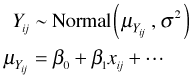
Let Y be a positive, continuous response variable. For instance Y might denote biological size measured over time. If the full range of an organism's life span is under consideration some values of Y will be near zero (occurring early in the organism's life span), and others will be far removed from zero (occurring later in the life span). Suppose we fit an ordinary regression model in which we assume that the i^th individual's mean size varies linearly on the j^th occasion with a time-dependent predictor x_ij (such as its age) and perhaps other predictors.

This is probably a silly model. Because the normal distribution is an unbounded distribution, it allows Y to take negative values. The probability that Y is negative could be non-negligible for small predicted values of the mean. The presence of a lower bound of zero will also restrict the variability of the response. If Y is predicted to be close to the boundary for some values of x, its overall distribution will tend to be heteroscedastic as a function of x. Because the normal distribution for Y assumes the variance is constant and independent of the mean, heteroscedasticity indicates yet another problem with a normal model for these data.

Transforming the response variable

The classical approach to handling this problem would be to transform the response and assume that the transformed variable has a normal distribution with constant variance. For the scenario I've described a common choice would be a log transformation. Thus we would assume

The notation used in the regression equation is meant to indicate that we are modeling the mean of log Y rather than mean of Y. In the first regression model the regression equation yields the mean of the response on the original raw scale of the response. In the transformed regression model the regression equation yields the mean of the response on a log scale. These are obviously not the same. Furthermore there is no way to transform a mean on the log scale into a mean on the raw scale.

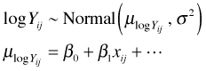
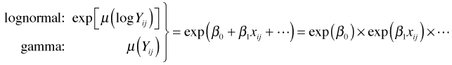
Although exponentiating the regression equation for log Y does yield a value that is on the scale of the raw response, it does not yield the mean of the response on the raw scale. The problem mathematically is that the "mean function" and the exponential function don't commute and so the exponential and logarithm operations can't cancel each other out.

On the other hand, because

1. the mean and median of a normal distribution are the same, and
2. the logarithm is a monotonic transformation,

exponentiating the regression equation for mean log Y does yield an expression for the median response on the raw scale (but not the mean).

Choosing a probability distribution and a link function

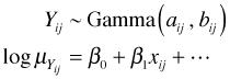
The modern approach to handling data of this sort is to choose a probability distribution that is more appropriate for a positive, continuous response variable. (In reality this is not really so different from the classical approach. Log-transforming a response and assuming the log is normally distributed is equivalent to assuming that the original response variable has a lognormal distribution. The lognormal distribution is a probability distribution that is appropriate for a positive, continuous response variable.) In the generalized linear model framework a reasonable choice for the probability distribution would be a gamma distribution.

where a > 0 and b > 0. The parameters a and b are related to the mean and variance of the gamma distribution as follows.

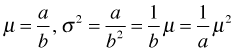
Because a and b are positive, the mean of the gamma distribution is positive. To guarantee that the regression equation only returns positive values for the mean, the usual approach is to formulate a regression equation for log μ rather than μ. The log function used in this way is referred to as a link function because it links the mean of a gamma distribution to the linear predictor of the regression model.

Typically one of a or b, usually b, is treated as a constant.

Unlike the case of a log-transformed regression model, when a log link is used it is possible to recover the mean on the raw scale by exponentiating both sides of the regression equation.

So, by choosing a log link function and a gamma distribution for positive data we do end up with a model for the mean on the raw scale. This makes using a generalized linear model an attractive alternative to transforming the response variable.

One possible drawback with both a log transformed response and the use of a log link function is that in the end our predictors have multiplicative effects rather than additive ones on the scale of the original response.

Marginal and subject-specific interpretations of a mixed effects model

Identity link

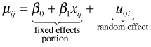
A normal random intercepts model with an identity link is a multilevel model with two levels. We have

Here i denotes the level-2 unit (the cluster) and j denotes the observation on that level-2 unit. The model for the mean is the following.

So the mean consists of two components: a fixed effects portion and a random effects portion. The fixed effects portion can be interpreted in two distinct ways.

1. The fixed effects portion corresponds to the mean response of an individual for whom u_0i = 0. So, the fixed effects portion is the response of a typical individual, one that lies at the center of the random effects distribution. This is a subject-specific interpretation of the mixed effects model because it focuses on the behavior of a specific subject.
2. A second interpretation can be obtained by averaging across subjects in the equation for the mean. Formally this is done by integrating both sides of the equation with respect to the probability density,, of the random effects distribution. In the examples we've considered is a normal distribution.

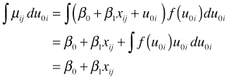
The last step follows because the expectation (mean) of the random effects distribution is zero by assumption, . Thus we see that the fixed effects portion is also the average mean across subjects. This is referred to as the marginal interpretation of the mixed effects model. When the data are a random sample from a known population the marginal interpretation of the fixed effects portion is also called the population-averaged interpretation.

So, in summary, in a mixed effects model with an identity link there are two distinct models for the mean. There is the

1. marginal (population-averaged) model: , and the
2. subject-specific model:

These models are different except for one particular subject, namely a subject for whom u_0i = 0. In a similar vein the marginal model has both

1. a marginal interpretation (it is the average across individuals) and
2. a subject-specific interpretation (it is the mean of the individual at the center of the random effects distribution).

When we use an identity link we get both of these interpretations for the mean response. When the link function is something other than the identity link, the marginal interpretation of the mean breaks down.

Logit link

Consider a generalized linear mixed effects model (GLMM) in which the response has a binomial distribution and we model the probability of success with a logit link. For simplicity we use the same random intercepts model that was used for the normal model with identity link.

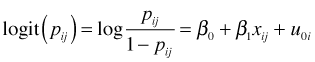
Let's try once again to interpret the fixed effects component of the model. With a logit link for the mean we can apply the inverse logit function

to express the mean, the probability of success p_ij, as a function of the linear predictor.

Subject-specific interpretation

If we set u_0i = 0 in the logit link equation we see that the fixed effects portion, , represents the logit of an individual that lies at the middle of the random effects distribution on the logit scale.

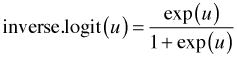
Inverting the logit yields

In the subject-specific interpretation the inverse logit of the fixed effect portion is the probability of success of an individual that lies at the middle of the random effects distribution on a logit scale.

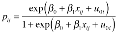
To obtain the marginal interpretation we need to average across individuals, i.e., average over the random effects distribution. Thus we have

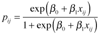
So the fixed effects portion represents the average individual logit. What is its relationship to the average probability of success, i.e., the average value of p? Now we're stuck because the inverse logit of this expression is not equal to the average value of p.

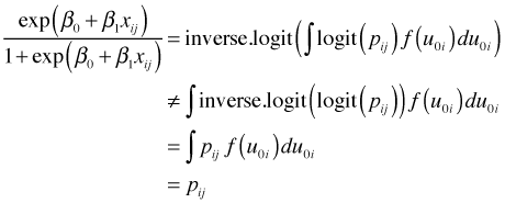
The problem is the same one we had when we tried to back-transform the regression equation for the mean of a transformed response variable. The operation of taking the mean (the integral in this case) lies between the link function and its inverse, and so the logit and inverse logit do not formally cancel. As a result back-transforming the marginal logit of p does not yield the marginal value of p.

The use of the logit link function in a mixed effects model messes up the marginal interpretation of the fixed effect terms. With an identity link the regression mean has both a subject-specific interpretation and a marginal interpretation. When the link is not the identity, the back-transformed linear predictor still has a subject-specific interpretation, but not a marginal one. This means that the p that corresponds to the mean of logit(p) is not also the mean of p.

Problems with the subject-specific interpretation of a mixed effects logit model

Without a true marginal interpretation for the fixed effects portion of the mixed effects model, is the subject-specific interpretation enough? In most cases the answer is no. Consider a hierarchical logit model that contains both a level-1 (individual-level) predictor x and a level-2 (group-level) predictor z.

• The coefficient β₁ of x has a useful subject-specific interpretation because x can vary within a subject. For a given subject (a fixed value of u₀) if the variable x increases by one unit then the logit increases by β₁ units. exp(β₁) is the amount the odds of success is increased by a one unit increase in x.
• The coefficient of z on the other hand does not have a sensible subject-specific interpretation. The variable z is constant within a subject, so unlike x it cannot change when u₀ is held fixed. In order for z to change we need to switch to another subject, but if we do so the random effect u₀ also changes. As a result the observed change in the logit will be due to both a change in z and a change in u₀. To obtain a subject-specific interpretation of β₂ we are forced to concoct a rather fanciful scenario. If two individuals have exactly the same value of the random effect u₀ but their value of z differs by one unit, then β₂ tells us how much the logit is predicted to differ between those two individuals. Alternatively exp(β₂) is the ratio of their odds of success.

Even if we're willing to engage in the mental gymnastics needed to give a subject-specific interpretation to the coefficients of group-level variables, we still can't treat the coefficient as indicating a change in the population average. The logit transformation maps proportions in the interval (0, 1) to logits on the interval (–∞, ∞). If the distribution of a set of proportions is skewed (lots of values near zero or lots of values near one), the distribution of the logits will be even more skewed. This means that if we average the logits and back-transform this average to a proportion we end up with a value that is more extreme (closer to 0 or closer to 1) than if we just averaged the proportions. The upstart is that the marginal value and the subject-specific value of the regression coefficient of a group-level predictor in a logit model can be widely different.

The difference in the subject-specific and marginal interpretations of mixed effects models with non-identity links has received extensive treatment in the statistical literature. A discussion of these issues aimed at ecologists can be found in Fieberg et al. (2009).

Cited references

• Fieberg, John, Randall H. Rieger, Michael C. Zicus, and Jonathan S. Schildcrout. 2009. Regression modelling of correlated data in ecology: subject-specific and population averaged response patterns. Journal of Applied Ecology 46(5): 1018–1025.

Course Home Page