Lecture 15—Monday, February 13, 2012

Topics

• The problem of correlated data
  • Why can't we ignore correlation in data?
  • The special characteristics of temporal data
• The mathematics of generalized least squares (GLS)
  • Overview of least squares (OLS)
  • Generalized least squares (GLS) for correlated data
• Using the ACF to identify the form of temporal correlation
  • Definition of the ACF
  • Using the ACF

The problem of correlated data

We'll spend the next three weeks discussing methods for handling correlated data. We focus on three distinct approaches.

1. Generalized least squares (GLS). This is a generalization of ordinary least squares in which we explicitly account for correlation in data. For it to work we need to have enough data to be able to accurately estimate correlations. For this reason generalized least squares is especially suitable for temporal data that consist of long time series. Because it's least squares, it is most appropriate when the response variable can be assumed to be normally distributed.
2. Mixed effects models. This is an omnibus approach and is especially appropriate when the presence of correlation is obvious, but the exact form of the correlation is not. Generally speaking one often uses a mixed effects model if it's felt that doing something, even if it's crude, is better than doing nothing at all. With temporal data mixed effects models are especially suitable for short time series where there isn't enough data to accurately determine the exact nature of the correlation structure. A serious problem with mixed effects models is that for non-normal response variables, particularly binary data with a logit link, their interpretation is problematic and counter-intuitive.
3. Generalized estimating equations (GEE). GEE can be considered analogous to GLS for non-normal responses. It assumes that observations come in clusters such that observations from the same cluster are correlated but observations from different clusters are not. As is the case with GLS in GEE the correlation is modeled explicitly.

This list leaves out a lot of other more specialized approaches, particularly those for dealing with specific sorts of spatial correlation. Examples include CAR (conditional autoregressive) and SAR (simultaneous autoregressive) models that are complicated instances of mixed effects models when observations have an identifiable neighborhood structure. These are both best handled from a Bayesian perspective.

Why can't we ignore correlation in data?

If we are taking a likelihood perspective then the likelihood we've been formulating is wrong if the data are truly correlated. In the discrete case the likelihood of our data under a given model is the joint probability of obtaining our data under the given model.

Now if x₁, x₂, ... , x_n are a random sample then the observations are independent and their joint probability can be written as a product of their identical marginal distributions.

Accordingly the log-likelihood is the sum of individual log probabilities. This is the scenario we've assumed in order to obtain the parameter estimates of generalized linear models.

If the data are not independent then the above factorization is invalid. As a result the likelihood and AIC are wrong, the results of model selection may be incorrect, and the parameter estimates and their standard errors may be affected. If we use least squares to estimate the model and we have normally distributed response, then the parameter estimates we obtain will still be correct but the reported significance tests for those parameters will be wrong. This reasons for this are the following.

• The reported standard errors will be too small (under the assumption that the observations are positively correlated—the usual case for temporally correlated data). Thus we can obtain significant results when we should not.
• The sample size is inflated. If we have a random sample with n = 100 then we have 100 distinct bits of information. If on the other hand the data in our sample are correlated then from an information-theoretic perspective some of the information is redundant and we really have less than 100 bits of information. So, the actual sample is n < 100. This in turn affects standard errors and the degrees of freedom for our tests.

It's worth noting that most ecological data sets possess spatial and/or temporal extent and thus will be correlated to some degree.

When we assume independence in formulating the likelihood, the independence is conditional on the values of the model parameters. In a regression model estimates of the parameters are functions of the model predictors. Consequently if the predictors in the model also vary both spatially and temporally, we expect that at least some if not all of the correlation in the response variable will be explained by the regression model. Given this our focus here will be the following. After fitting the best regression model we can, what should we do about any lingering correlation that remains in the response variable?

The special characteristics of temporal data

To introduce methods for dealing with correlated data we will focus on temporal data because temporal data are the easiest to model.

1. Temporal correlation is one-dimensional and unidirectional. We only have to worry about the effect that the past has on the present, not vice versa.
2. The toolbox for the analysis of temporal data is quite full. Time series analysis has long been an important subject in financial analysis, for example in the prediction of future stock behavior. As a general rule when there is money to be made, the available analytical tools will typically be quite good.

The mathematics of generalized least squares (GLS)

Because it generalizes ordinary least squares, generalized least squares (GLS) is largely restricted to situations in which a normal distribution makes sense as a probability model for the response. For non-normal correlated data the choices are murkier, so for the moment we'll focus exclusively on regression models with a normally distributed response. Generalized least squares requires us to formulate a specific model for the variances and covariances of our observations. This is not difficult with temporal data because there are some obvious choices. For this reason we will focus on analyzing temporal data using GLS.

Overview of ordinary least squares

In matrix notation, the ordinary regression problem can be written as follows.

Here

• y is an n × 1 vector of values of the response variable.
• X is an n × p matrix called the design matrix. Each column corresponds to a different regressor and each row corresponds to the values of the regressors for a different observation.
• β is a p × 1 vector of regression parameters.
• ε is an n × 1 error vector.

The method of least squares yields an explicit formula for the estimates of the components of β.

The least squares solution doesn't make any distributional assumptions but to obtain statistical tests and confidence intervals we need to assume a probability distribution for the response vector y. Least squares lends itself to assuming a normal distribution for y which we can write as follows.

Here I is the n × n identity matrix, a matrix of zeros except for ones on the diagonal. This is the matrix formulation of independence for a normally distributed response. We can also express this assumption in terms of the error vector of the regression equation.

This assumption coupled with the least squares solution leads to the theoretical distribution of the regression parameters β (normal distribution) and an explicit formula for their standard errors.

Generalized least squares (GLS) for correlated data

Generalized least squares (GLS) generalizes ordinary least squares to the case where the residuals have a normal distribution with an arbitrary covariance matrix Σ.

For convenience we will write the covariance matrix in the form . It turns out that not every matrix is a covariance matrix. Covariance matrices are rather special.

1. Covariance matrices are positive definite. Positive definiteness is the matrix version of the scalar notion of being positive.
2. Covariance matrices admit a square root decomposition referred to as the Cholesky decomposition. This means that we can write

for some nonsingular, symmetric matrix P. P act like the square root of V and is sometimes called a square root matrix.

It turns out that

so that we can uncorrelate the errors with an appropriate transformation, namely premultiplying the response vector by P^–1. So, suppose we have the following generalized regression model.

We premultiply both sides of the regression equation by P^–1 to obtain the following.

where now . This is just the ordinary least squares problem again with the variables and matrices relabeled. The formula for the solution was given above.

So as was the case with ordinary least squares we end up with an exact formula for the regression parameters, this time in terms of the design matrix and the unscaled covariance matrix V. Unfortunately the formula requires that we know V, so typically we'll need to estimate it first.

To make this problem feasible and to avoid overparameterization, the usual approach is to assume that V has a very simple form, a correlation structure that is based on a small number of parameters, and to jointly estimate the regression parameters and the covariance parameters. There are specific algorithms for special correlation structures, but a general approach is to use maximum likelihood estimation. This can be done by using the above solution for β (as well as the MLE expression for σ) and treating the log-likelihood as a function to be maximized over the unknown correlation parameters.

Using the ACF to identify the form of temporal correlation

To implement generalized least squares we need to choose a parametric form for the matrix V. If we assume that the residuals all have the same variance, then the matrix V is the correlation matrix of the residuals. For temporal data the primary tool for identifying reasonable models for the correlation is the empirical autocorrelation function (ACF).

Suppose that a regression model has been fit to temporal data, consisting of either a single time series or a set of time series (repeated measures on different units), and that the standardized residuals have been extracted from the model.

Here . We make the following what are called stationarity assumptions about the residuals.

1. Their mean is not changing. If we've modeled the regression relationship correctly then the model errors should have mean zero.
2. The correlation between the residuals is only a function of their relative temporal position and is not related to their absolute temporal position.

As a consequence of the stationarity assumptions, especially (2), we can define the residual autocorrelation at various lags by considering all the pairs of residuals that are the same number of time units apart (Fig. 1). Lag 1 observations are all pairs of observations that are one time unit apart, lag 2 observations are all pairs of observations that are two time units apart, etc.

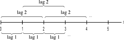
Fig. 1  Observations that are 1, 2, … time units apart

Definition of the ACF

We assume that the residuals are sorted in time order. If the data consist of multiple time series that correspond to different observational units, then within each observational unit the residuals should be sorted in time order. For a single time series of length n we define the autocorrelation at lag as follows.

If we have M different time series of varying lengths then the average is taken over all the individual time series.

Here is the number of terms in the numerator sum (the total number of residual pairs a distance of time units apart) and N(0) is the total number of residuals. The autocorrelation function (ACF) is the lag correlation, , treated as a function of the lag .

Observe that the formula for the lag autocorrelation is just a special case of the usual Pearson correlation formula except that here the means are zero and a different numbers of terms contribute to the numerator and denominator expressions.

Using the ACF

The autocorrelation function is usually examined graphically by plotting against in the form of a spike plot and then superimposing 95% (or Bonferroni-adjusted 95%) confidence bands. We expect with temporally ordered data that the correlation will decrease with increasing lag. Fig. 2 shows a plot of the ACF that is typically seen with temporally correlated data. Here the correlation decreases exponentially with lag.

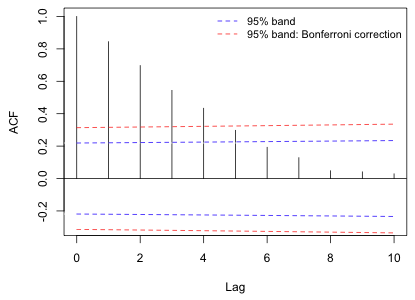
Fig. 2  Display of an ACF with 95% confidence bands

The confidence bands for the ACF are calculated using the following formula.

Here z(p) denotes the quantile of a standard normal distribution such that P(Z ≤ z(p)) = p. For an ordinary 95% confidence band we would set α* = .05. For a Bonferroni-corrected confidence bound in which we attempt to account for carrying out ten significance tests (corresponding to the ten nonzero lags shown in Fig. 2) we would use α* = .05/10.

Course Home Page