Lecture 23 (lab 8)—Friday, March 2, 2012

Topics

• Background on the data
• Generalized estimating equations using the gee package
• Choosing a correlation structure
• Generalized estimating equations using the geepack package
• A binary mixed effects model
• Comparing marginal and subject-specific models
• Checking the correlations for feasibility
• Cited references

R functions and commands demonstrated

• gee (from gee) for fitting GEE models.
• geeglm (from geepack) for fitting GEE models.
• lmer (from lme4) sets up and fits generalized linear and nonlinear mixed effects models.
• paste concatenates text strings together.

R function options

• corstr= (argument to gee and geeglm) for defining the correlation structure within groups in a GEE model.
• id= (argument to gee and geeglm) is used to identify the grouping variable in a GEE model.
• Mv= (argument to gee) for specifying the order of an autoregressive process or the order of a stationary or nonstationary M dependent correlation matrix.
• scale.fix= (argument to gee and geeglm) when set to TRUE causes the scale parameter to be fixed (by default at 1) rather than estimated.
• sep= (argument to paste) identifies the value that should be used to separate the concatenated text strings.
• waves= (argument to geeglm) names a positive integer-valued variable that is used to identify the order and spacing of observations within groups in a GEE model. This argument is crucial when there are missing values and gaps in the data.
• zcor= (argument to geeglm) is used to specify the entries of a correlation matrix to accompany corstr="fixed".

R packages used

• gee used for the function gee to fit GEE models.
• geepack used for the function geeglm to fit GEE models.
• lme4 used for the function lmer to fit generalized linear mixed effects models.

Background on the data

To illustrate the process of fitting GEE models in R, we use some binary data analyzed in Fieberg et al. (2009). The goal of their study was to relate nest occupancy by mallards (a binary response) to surrounding land use characteristics and the type of nesting structure that was provided. The authors provide R code for their analysis in a supplemental document. As we'll see, the authors made some mistakes in fitting their models.

Individual nests were observed repeatedly over time and at each time point the nest was classified as occupied (nesting2 = 1) or unoccupied (nesting2 = 0) by mallards. If the nest was occupied by a species other than mallard, no data were recorded or nesting2 was assigned a missing value, NA. The available predictors include the following.

• year: the year of the observation (1997, 1998, 1999)
• period: the seasonal observation period (1, 2, 3, 4)
• deply: nest structure type (1 for single cylinder, 2 for double cylinder)
• size: the size of the wetland in which the nest structure was located
• rblval: a measure of visual obstruction around the nest

A variable strtno identifies the site at which measurements were made. Of these variables, deply and size were constant for a given nest site, while year, period, and rblval varied over time.

I load the data that I previously downloaded to my laptop and display part of the records for the first two nesting sites in the data set.

The largest number of observations per nest is 12, but some of the nests have fewer than 12 observations.

I examine the data from some of the nests with fewer than the maximum number of observations.

Nests 4 and 30 are missing the last year of data, 1999. Nest 32 is missing the first year of data but also seasons 2 and 3 in 1998. Because values for the predictors were recorded at these two times but the response, nesting2, is recorded as missing (NA), we conclude that the nest was being occupied by a different species. The unbalanced data and the presence of missing values in some of the records will have an impact on the way models will need to be fit.

Generalized estimating equations using the gee package

The model Fieberg et al. (2009) choose to fit in all of their examples is one that includes main effects for the five predictors year, period, rblval, deply, and size, a quadratic term for size, and interactions between period and year as well as between rblval and period. The variables year, period, and deply are recorded as numeric variables in the data set but need to be treated as factors in the model. In R notation the basic logistic regression model that we'll use is the following.

R has two packages that fit GEE models: the gee package and the geepack package. Because there are slight differences in the algorithms used by these packages, the results returned by them are not identical. Although there is considerable overlap between the two packages, the geepack package offers a number of advantages if there are missing data.

We'll start with the gee package. The function in this package for fitting GEE models is the gee function. In addition to the model syntax shown above gee requires two additional arguments:

1. id= which is used to identify the grouping variable in the data set (within which observations are correlated). For the sm data set the grouping variable is strtno.
2. corstr= which is used to identify the correlation structure within groups (id).

The gee package offers the following correlation structures for the corstr argument.

• "independence": the observations within the groups are uncorrelated.
• "exchangeable": each pair of observations in a group has the same correlation.
• "unstructured": each pair of observations in a group is allowed to have a different correlation.
• "AR-M": this is used to fit an autoregressive structure. To obtain a specific autoregressive structure requires the additional argument Mv. For example corstr="AR-M", Mv=1 yields an AR(1) structure, while corstr="AR-M", Mv=2 yields an AR(2) structure.
• "non_stat_M_dep": stands for nonstationary M-dependent and generates a banded correlation matrix. It also requires the Mv argument to denote the number of nonzero off-diagonal bands that are to be estimated. Like "AR-M", "non_stat_M_dep" assumes there is a natural order to the data. Like "unstructured", "non_stat_M_dep" allows the entries within the each nonzero band to be different. As an example corstr="non_stat_M_dep", Mv=1 would correspond to the following correlation matrix for a group of size 4. Here α, β, and γ are parameters that need to be estimated.

• "stat_M_dep": stands for stationary M-dependent and generates a banded structure. It also requires the Mv argument which denotes the number of nonzero bands to include. Like "AR-M", it assumes there is a natural order to the data but differs from "AR-M" in that the entries in different bands are unconnected to each other. Within a band all the entries are assigned the same correlation parameter (unlike "non_stat_M_dep"). Mathematically the correlation matrix that is produced is called a Toeplitz matrix. For example, corstr="stat_M_dep", Mv=2 for a cluster of size 4 would yield the following correlation matrix. Here α and β are parameters that need to be estimated.

Because we are working with binary data we need to include one further argument: scale.fix=T. This option causes the scale parameter to be fixed at its default value of 1 rather than estimated. Omitting this argument and allowing gee to estimate the scale parameter generates a quasibinomial model, which is an adjustment for overdispersion. Because binary data cannot be overdispersed, a quasibinomial model is never appropriate for binary data. For true binomial (non-binary) data and Poisson data we would typically let this argument take its default value of F so that a scale parameter is estimated. Note: Specifying corstr="independence" and scale.fix=F yields the same result as fitting the model with glm and specifying family=quasibinomial.

To fit a GEE model with an exchangeable correlation structure to the nesting data we would enter the following.

The summary function applied to this object provides information about the model fit. I extract some of its components individually in order to reduce the amount of output that is displayed. First I examine the scale parameter and the estimated correlation matrix.

The scale parameter was not estimated but was fixed at 1, which is correct for binary data. The correlation between observations within a group is estimated to be 0.13. Because we specified an exchangeable correlation structure, this correlation is the same for every pair of observations within the group. What's displayed above is the full 12 × 12 correlation matrix for the largest group.

Next I examine the coefficient table of parameter estimates.

The multiple standard error columns deserve comment. It was mentioned in lecture 22 that GEE software routinely produces two standard error estimates: a naive (or model-based) estimate and a robust (or sandwich) estimate. These are what are displayed here. The naive estimate is the standard error under the assumption that the correlation matrix has been correctly specified and estimated. The robust estimate modifies the naive estimate by a term that depends on the covariance of the model residuals across groups. It is robust in the sense that using it allows one to draw correct inferences from the data even if the correlation model was incorrectly specified.

Although no p-values are shown, the reported z-statistics can be treated as standard normal random variables and significance tests carried out in the usual fashion. Based on the output it appears that our conclusions would be the same regardless of the standard error estimates we use.

Choosing a correlation structure

The subject of choosing a correlation structure in GEE models was discussed in lecture 22. A good starting point is to pick a correlation structure that makes sense given the nature of the data. Because these are repeated measures data, an exchangeable or an AR(1) structure are good choices. Choosing correlation structures such as unstructured and nonstationary M-dependent would be unmotivated here without additional information about the data. It is always useful to fit an independence model to serve as a reference. The next two runs fit an independence model and an exchangeable correlation model.

Because there are missing data and gaps in the temporal series of measurements, any correlation model fit with the gee function that depends on the order of the data will be incorrect. The gee function assumes that the non-missing observations in a group start at time = 0 and are then listed consecutively. With the gee function there is no way to indicate the presence of gaps in a time series. On the other hand the geeglm function in the geepack package doesn't have this shortcoming as will be explained below. Fieberg et al. (2009) fit all their models using the gee package but overlooked this problem. Hence the results they report for an AR(1) model fit are wrong.

Here's how one would ordinarily fit an unstructured, AR(1), stationary M-dependent, and nonstationary M-dependent model with the gee function. Because the results are wrong for these data I won't bother to examine the output from these models.

To compare models using QIC or CIC we need to write our own code to calculate these statistics. A function that works with gee output is shown below.

This function is available from the class web site. To use the function we need to specify two arguments: the model of interest (1st argument) as well as well as the independence model (2nd argument). Below I use the function to calculate QIC and CIC for the independence and exchangeable correlation models.

Both QIC and CIC rate the exchangeable model as best.

As was discussed in lecture 22 we can also use the naive and robust variance estimates to select a correlation model. The model whose robust variance estimates most closely resembles its naive variance estimates is the better correlation model. For this we can focus only on the variance estimates or we can use the entire variance-covariance matrix. The square roots of the variances can be extracted from the summary table. To obtain a single summary statistic for this comparison we might sum the absolute value of the differences of the variances.

Perhaps a better single summary statistic for this comparison is to use the entire parameter covariance matrix rather than just the variances. I sum the absolute differences between the naive and robust covariance matrices.

Both statistics select the exchangeable structure.

Generalized estimating equations using the geepack package

The geepack package can also be used to fit GEE models in R. It's primary advantage over the gee package is that it has a waves argument that can be used to identify the order of observations within groups making it possible to fit temporal correlation models to data sets with missing values. The primary disadvantage of the geepack package is that it provides fewer correlation structures, (currently only independence, exchangeable, unstructured, AR(1), and user-defined), although it is possible to define some additional structures as explained in Halekoh et al. (2006). The geepack package also provides a method for the anova function that can be used to carry out multivariate Wald tests.

First we need to create a variable for the waves argument—an integer-valued variable that reflects the order of the observations in groups so that the proper observations in different groups get matched up correctly. For the current data set we can accomplish this by pasting together the values of the variables year and period. The paste function concatenates text strings together separated by the value specified in its sep argument. We then convert the created text to a factor and finally use as.numeric to extract the numeric values of that factor, in this case the numbers 1 through 12.

We only need the waves argument for the unstructured and AR(1) correlations, but it doesn't hurt to include it in all the model calls. The function in the geepack package that fits GEE models is geeglm. The syntax is the same as for the gee function except that AR(1) is specified as corstr="ar1". Fitting an "unstructured" correlation matrix can be very resource-intensive and for these data causes R to crash, so we skip it. The independence, exchangeable, and AR(1) correlation models are fit as follows.

To compare these models we need to modify our QIC function so that it works with geeglm output. The function is shown below.

This function is also available from the class web site. Applying the function to the three models we have fit yields the following.

The exchangeable model ranks best using either CIC or QIC. The summary table of this model is shown below.

 Coefficients:
                                 Estimate  Std.err  Wald Pr(>|W|)   
(Intercept)                      -3.63025  0.63152 33.05    9e-09 ***
factor(year)1998                  1.01778  0.36533  7.76   0.0053 **
factor(year)1999                  0.95134  0.30565  9.69   0.0019 **
factor(period)2                   1.28438  0.70682  3.30   0.0692 . 
factor(period)3                   2.43981  1.79132  1.86   0.1732   
factor(period)4                   4.84071  2.52702  3.67   0.0554 . 
factor(deply)2                   -0.01573  0.29467  0.00   0.9574   
rblval                            3.90822  1.66698  5.50   0.0191 * 
size                              0.22636  0.05514 16.85    4e-05 ***
I(size^2)                        -0.00715  0.00222 10.34   0.0013 **
factor(year)1998:factor(period)2 -1.84861  0.57064 10.49   0.0012 **
factor(year)1999:factor(period)2 -1.20950  0.45579  7.04   0.0080 **
factor(year)1998:factor(period)3 -1.47907  0.82720  3.20   0.0738 . 
factor(year)1999:factor(period)3 -1.12472  0.79685  1.99   0.1581   
factor(year)1998:factor(period)4 -1.61419  0.69213  5.44   0.0197 * 
factor(year)1999:factor(period)4 -1.25735  0.63192  3.96   0.0466 * 
factor(period)2:rblval           -2.40517  2.22897  1.16   0.2806   
factor(period)3:rblval           -5.11459  2.50854  4.16   0.0415 * 
factor(period)4:rblval           -6.02830  2.04198  8.72   0.0032 **
---
Signif. codes:  0 ‘***’ 0.001 ‘**’ 0.01 ‘*’ 0.05 ‘.’ 0.1 ‘ ’ 1

Scale is fixed.

Correlation: Structure = exchangeable  Link = identity

Estimated Correlation Parameters:
      Estimate Std.err
alpha    0.124  0.0223
Number of clusters:   109   Maximum cluster size: 12

The display differs somewhat from what is produced by gee. Only one column of standard errors is shown. These correspond to the robust estimates of gee. The naive estimates are not shown. The robust or Huber sandwich estimator provides reasonable variance estimates even when the specified correlation model is incorrect. If the correlation model is nearly correct, so will be the naive standard errors, and robustification is unlikely to help much. So, unless you have strong reason to believe that the chosen correlation matrix is correct, it is recommended to always report the robust standard errors.

The column labeled Wald in the summary table is the square of the z-statistic reported by the gee function. Both the z-statistic and its square are variously referred to as Wald statistics. The square of a standard normal random variable is a chi-squared random variable with 1 degree of freedom, . So, the reported p-values are the upper tailed probabilities from a distribution and test whether the true parameter value is different from zero.

The naive variance-covariance matrix of the parameter estimates can be found as the vbeta.naiv component of the geese component of the model.

Using these standard errors Wald statistics can then be constructed by hand. The squared versions of the Wald statistics using the naive standard errors are shown below.

These can then be compared to the upper tail of a distribution to obtain p-values.

These are quite similar to the p-values reported using the robust standard errors.

As was discussed in lecture 22 we can also use the naive and robust variance estimates to select a correlation model. The model whose robust variance estimates most closely resembles its naive variance estimates is the better correlation model. To obtain a single summary statistic for this comparison I use the entire parameter covariance matrix and sum the absolute differences between the naive and robust covariance matrices.

The sum of the absolute differences between the naive and robust covariance estimates is smallest for the exchangeable correlation structure. This is consistent with the conclusions we drew using QIC and CIC.

To test whether a categorical predictor with more than two levels should be retained in a GEE model we need to test the entire set of dummy variables simultaneously as a single construct. The geepack package provides a method for the anova function that carries out a multivariate Wald test. (Remember, there is no likelihood associated with GEE models and hence no likelihood ratio tests.) When the anova function is applied to a single geeglm object it returns sequential Wald tests for individual predictors with the tests carried out in the order the predictors were listed in the model formula.

                            Df    X2 P(>|Chi|)   
factor(year)                 2  0.24    0.8872   
factor(period)               3 23.14   3.8e-05 ***
factor(deply)                1  0.02    0.8927   
rblval                       1  1.01    0.3147   
size                         1  7.57    0.0059 **
I(size^2)                    1  9.43    0.0021 **
factor(year):factor(period)  6 20.00    0.0028 **
factor(period):rblval        3  9.01    0.0291 * 
---
Signif. codes:  0 ‘***’ 0.001 ‘**’ 0.01 ‘*’ 0.05 ‘.’ 0.1 ‘ ’ 1

A binary mixed effects model

An alternative way to account for repeated measures is to fit a mixed effects model with random intercepts. This yields what's called a conditional model instead of the marginal model that we obtain with GEE. The parameters of a conditional model have a subject-specific interpretation rather than the population-average interpretation of a marginal model. Because logistic regression uses a nonlinear link function, the magnitudes of the estimated effects in marginal models will differ from those same effects estimated in conditional models. (See lecture 21.) In logistic regression the parameter estimates from a conditional model tend to be larger in magnitude (more positive or more negative) than the corresponding parameter estimates from a marginal model.

The lme4 package fits generalized linear mixed effects models (GLMM) and can be used to fit a random intercepts model to binary data. A brief explanation of the syntax used in this package was given in lecture 20.

For comparison I also fit an ordinary logistic regression model in which the repeated measures structure is ignored.

If we compare the AIC of the ordinary logistic regression model with that of the mixed effects logistic regression model we see that the AIC of the mixed effects model is lower indicating that it should be preferred. Thus we have evidence for observational heterogeneity, a conclusion that is consistent with the GEE model selection results that favored an exchangeable correlation structure over independence.

Comparing marginal and subject-specific models

Next I compare the parameter estimates from GLM, GEE, and GLMM.

From the output we see that the subject-specific (conditional) mixed effects model coefficients are larger in magnitude than the same coefficients from the population-averaged (marginal) GEE model. As was explained in lecture 21, the difference arises because averaging on a logit scale (conditional model) is not equivalent to averaging on the scale of the raw response (marginal model).

For these data the variables year, period, and rblval have clear subject-specific interpretations because they vary across observation times. On the other hand the variables size and deply do not have clear subject-specific interpretations because they are constant at each nest site. With size this doesn't matter too much because size is a control variable that is probably uninteresting on its own. On the other hand the variable deply (nest box type) is of some interest. For a subject-specific interpretation to make sense for deply we would need to be able to compare two individuals who are identical (have the same random effect) but occur in different nest box types.

Fig. 1 compares the subject-specific and population-average interpretations for the predictor rblval during period 1 of 1999 for a single cylinder nest (deply = 0) in a wetland of size = 0. The individual subject-specific curves that are displayed cover the complete range of random intercepts that were predicted. The pure fixed effects model corresponds to the center of this random effects distribution, u_i = 0, and so represents the typical individual, i.e., the average individual on a logit scale. As the plot shows this is quite different from the marginal model, which represents the average individual on a probability scale.

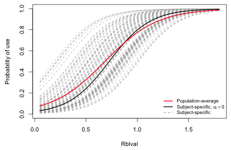
Fig. 1  Comparing subject-specific and population-average models

Checking the correlations for feasibility

As was discussed in lecture 22, the binomial distribution places constraints on the correlations that are possible. Because the mean and variance of binomial random variables are related, correlations between pairs of binomial random variables are related to their means, i.e., their joint probabilities. Prentice (1998) derived the following formula for the joint probability of the binary pair y_i and y_j.

This joint probability is non-negative when

Solving the inequality for r_ij yields the following bounds on the correlation depending on the possible values of the binary observations.

lower bound:   if y_i = 1 and y_j = 0 or y_i = 0 and y_j = 1

upper bound:   if y_i = 1 and y_j = 1 or y_i = 0 and y_j = 0

The following function calculates the set of lower bounds and upper bounds for a given entry in the working correlation matrix. It examines the predicted probabilities and observed binary values for all observations that contribute to that correlation matrix entry and returns the value of the bound that they provide. The function has five arguments.

1. A vector of predicted probabilities, the fitted values.
2. A vector of observed binary values.
3. A vector of values of the wave variable.
4. The value of the wave variable for the first observation, y_i.
5. The value of the wave variable for the second observation, y_j.

The two values of the wave variable determine the location of the entry in the correlation matrix.

To use this function we call it from a second function that then calculates the maximum lower bound and minimum upper bound on the correlation for a given correlation matrix entry.

To use this function efficiently we need to construct a matrix whose rows contain all the possible pairs of values of the wave variable. For the current data set where the wave variable takes values 1 through 12, there are = 66 pairs to consider. We can generate them all with a nested for loop.

The first 15 rows are shown below.

In the current data set the groups are unbalanced and the response variable has occasional missing values. Thus the returned fitted values and original response variable are of different lengths. To use them in the functions we first need to flesh out the data so that each group has 12 waves with missing values inserted for the waves that are not present.

With these preliminaries we can use the observed and fitted values to calculate bounds for each entry in the correlation matrix. I use sapply to move row by row through the matrix wave.mat extracting pairs of wave values that correspond to the different locations in the correlation matrix.

The first 8 lower and upper bounds are shown below.

With an exchangeable correlation matrix all the correlations are the same so we just need to be sure that this value lies within all 66 of the different lower and upper bounds we calculated. For more general correlation matrices we would need to match these bounds with the corresponding correlation matrix entries. The listed bounds correspond to the upper triangle of the correlation matrix listed by row or equivalently, the lower triangle of the correlation matrix listed by column. The following extracts the correlation matrix entries in the same order specified by the bounds.

Finally we can test that each estimated correlation lies within the calculated bounds.

So, the bounds are satisfied for all entries in the estimated exchangeable correlation matrix.

What should one do if one or more of the bounds are not satisfied? Ziegler and Vens (2010) argue that the corresponding correlation model should be rejected in this case. I think this position is too extreme. Typically the violation is minor in that only a small fraction of the joint probabilities are negative and often just barely so. In this case an argument could be made for just ignoring the problem. Probably a more honest solution is adjust the corresponding entry in the correlation matrix by moving it toward zero enough so that it now lies just inside the required bounds. This is an especially attractive option for unstructured correlation matrices where only a few entries are likely to be affected, less so for matrices that depend on a single parameter where changing one entry requires changing them all.

After making changes to the correlation matrix the GEE model can then be re-estimated treating the correlation matrix as fixed rather than a function of parameters that need to be estimated. In the geepack package this is accomplished by specifying corstr="fixed". The values in the lower triangle of the correlation matrix are entered into a vector where they are repeated as many times as there are groups in the data. This vector is then entered as the zcor argument of geeglm. An example appears in the help window for the geese function for the case of balanced data in which each group has the same number of observations. If the different groups have different numbers of observations then constructing the zcor object is more complicated. Furthermore, if the data set is even moderately large it's quite easy for geeglm to crash R, which it does with the current data set.

Cited References

• Fieberg, John, Randall H. Rieger, Michael C. Zicus, and Jonathan S. Schildcrout. 2009. Regression modelling of correlated data in ecology: subject-specific and population averaged response patterns. Journal of Applied Ecology 46(5): 1018–1025.
• Halekoh, Ulrich, Søren Højsgaard, and Jun Yan. 2006. The R package geepack for generalized estimating equations. Journal of Statistical Software 15(2).
• Prentice R. L. 1988. Correlated binary regression with covariates specific to each binary observation. Biometrics 44: 1033–1048.
• Ziegler, A. and M. Vens. 2010. Generalized estimating equations: Notes on the choice of the working correlation matrix. Methods of Information in Medicine 49: 421–425.

Course Home Page