The data for today's lecture are the coral extension rates that we previously examined in lecture 17. They consist of the annual growth rings from coral cores extracted from 13 Siderastrea siderea colonies inhabiting the outer (forereef, backreef) and nearshore reefs of the Mesoamerican Barrier Reef System in southern Belize. The R commands from lecture 17 that we used to read in and process the data are listed below.
The data frame that these commands generate is called ext.rates2.
This is a structured data set because although the observational units are the annual growth rings, the rings were obtained from a random sample of coral cores rather than a random sample of annual rings. Once a coral core was obtained it automatically brought with it all of the annual rings associated with that coral core. Such data are likely to exhibit observational heterogeneity because we have observations from different corals as well as multiple observations from the same coral core. Observations from the same core are likely to be more similar to each other than they are to observations from different cores.
In lecture 17 we fit a separate slopes and intercepts model using dummy variables to indicate the separate cores. We then accounted for temporal correlation in the separate time series of individual coral cores with generalized least squares. Today we replace the separate slopes and intercepts model with a random intercepts model and a random slopes and intercepts model. Because we are dealing with temporal data we will need to investigate whether an additional correlation model for the residuals is needed beyond the one that is contributed by the random effects.
There are two packages in R for fitting multilevel models. The older and more comprehensive package is nlme, an acronym for nonlinear mixed effects models. Its workhorse function is lme whose limitation is that it only fits normal-based models and is not designed to fit mixed effects models to data that are nonhierarchical. The newer R package for fitting mixed models is lme4 with its workhorse function lmer. The primary syntax differences between the lme and lmer functions lie in how the random effects component of the model is specified. The lme4 package fits generalized linear mixed effects regression models such as logistic and Poisson models and permits the inclusion of both hierarchical and crossed random effects. It currently lacks some of the nonlinear features and correlation functions of nlme. Because the lme4 package is under active development this situation may change.
Because the example we consider today has a normally distributed response, we will focus on the nlme package. The lme4 package will be considered again when we discuss generalized linear mixed effects models. The primary reference for the nlme package is Pinheiro and Bates (2000). A book is currently being written to describe the lme4 package. A preprint of the first five chapters is available here.
From a multilevel perspective, the coral cores data set consists of two levels. There is the annual ring level (level 1) and the core level (level 2). Any regression model that can be fit to a single level-2 unit, the individual core, is called a level-1 regression equation. The level-1 equation is our starting point for fitting a random intercepts model.
The random intercepts model is the simplest mixed effects model one can fit that still properly accounts for a data set's structure. For these data the variables that vary within a core are Ext.rate (the width of an individual ring) and Year (the time period during which that growth occurred). Thus the following regression equation could be fit separately to each individual coral core.
![]()
where ![]() . Here i denotes the coral core and j denotes a specific annual ring within that coral core. This is a level-1 equation. The equation says the width of the rings varies linearly with year. Because both β0i and β1i have subscripts i, each can potentially have different values for different coral cores.
. Here i denotes the coral core and j denotes a specific annual ring within that coral core. This is a level-1 equation. The equation says the width of the rings varies linearly with year. Because both β0i and β1i have subscripts i, each can potentially have different values for different coral cores.
In the random intercepts model we allow the intercept β0i to vary, but β1i is treated as a constant that is common to all of the cores.
where ![]() . Here u0i denotes how much coral core i deviates from the population average intercept β0. The random intercepts model formulated as a multilevel model can be written as follows.
. Here u0i denotes how much coral core i deviates from the population average intercept β0. The random intercepts model formulated as a multilevel model can be written as follows.
where ![]() . To understand how the R specification of this model works we need to substitute the level-2 equation into the level-1 equation to obtain the composite equation.
. To understand how the R specification of this model works we need to substitute the level-2 equation into the level-1 equation to obtain the composite equation.
From the composite equation we can directly construct the corresponding R code for fitting this model. The function in the nlme package for fitting linear mixed effect models is lme.
random=~"random variable"|"structural variable"
Observe that the response is not specified in the random part so the model statement begins with just a ~. Because the level-2 equations (one in our case) only include a random effect in the intercept equation, the intercept is identified as the only predictor on the right hand side of the model expression in the random= argument, random=~1. Another way to understand the origin of 1 in the random argument is that in the composite model we can think of
as being a coefficient multiplying the intercept, which is denoted by 1. Finally the vertical bar is used to separate the model specification from the structural specification. The variable Core is listed as the variable that defines the level-2 units.
The summary output from the random intercepts model is displayed below.
Random effects:
Formula: ~1 | Core
(Intercept) Residual
StdDev: 0.08384704 0.1203458
Fixed effects: Ext.rate ~ Year
Value Std.Error DF t-value p-value
(Intercept) 2.0263400 0.4010847 753 5.052150 0e+00
Year -0.0008155 0.0002023 753 -4.030118 1e-04
Correlation:
(Intr)
Year -0.998
Standardized Within-Group Residuals:
Min Q1 Med Q3 Max
-3.5820921 -0.6203362 -0.0555163 0.5814467 3.2817378
Number of Observations: 767
Number of Groups: 13
I've highlighted the information of interest to us.
Variance components are extracted from the model with the VarCorr function.
What's reported in the first column are the squares of the values reported in the summary table, so these are variances. From the output we determine that ![]() = 0.0070 and
= 0.0070 and ![]() = 0.0145. It turns out that output from VarCorr is a matrix of character strings.
= 0.0145. It turns out that output from VarCorr is a matrix of character strings.
So if we want to use the values from VarCorr directly in calculations we need to convert them first to numbers with the as.numeric function.
Previously we've used the coef function to extract the parameter estimates from regression objects. With an lme object there are three functions available for this purpose: coef, fixef, and ranef. The fixef function returns the fixed effect parameter estimates from an lme model. In model1 these are the estimates of the parameters we labeled β0and β1.
The ranef function returns predictions of the random effects for each of the structural units in our model. The structural units are the individual cores. The random effects are the terms we've been labeling ![]() . As was explained in lecture 19, the random effects are not parameters that are estimated when fitting the model, instead they are obtained after the fact using the estimates of the regression parameters and the variance components that were obtained. These estimates are referred to as empirical Bayes estimates, also called BLUPs (best linear unbiased predictors).
. As was explained in lecture 19, the random effects are not parameters that are estimated when fitting the model, instead they are obtained after the fact using the estimates of the regression parameters and the variance components that were obtained. These estimates are referred to as empirical Bayes estimates, also called BLUPs (best linear unbiased predictors).
The coef function combines the fixed effects with the random effects. It returns the random intercepts ![]() in column 1 as well as the fixed effect coefficient β1 in column 2. Notice that the random intercepts vary by core while the fixed coefficient is constant across all cores.
in column 1 as well as the fixed effect coefficient β1 in column 2. Notice that the random intercepts vary by core while the fixed coefficient is constant across all cores.
We obtain predictions of the mean for individual observations in an ordinary regression model by using the values of the predictors for those observations in the regression equation. With a random intercepts model there are two different predictions for the mean that we could calculate. There is the prediction that includes only the fixed effect estimates, referred to as the population average value, and a prediction that includes both the fixed effects and the random effects, called the subject-specific value.
We obtain these predictions by including the level argument in the predict function and assigning it the value 0 (population average) or 1 (subject-specific).
Observe that the difference between the population average and subject-specific predictions is equal to the random intercept for that core.
Because the random intercepts model yields a different subject-specific model for each core, an obvious way to display the model graphically is as a lattice graph. Because the observations were previously sorted in date order within each core we can graph the models by connecting the predicted values with line segments. In order to obtain the correct subject-specific predictions for each core we need to include the subscripts key word as an argument to the panel function and then use it in specific panel function calls to select the appropriate observations. In the code below the key argument is used to create a legend.
The key argument is mostly self-explanatory although a bit convoluted.
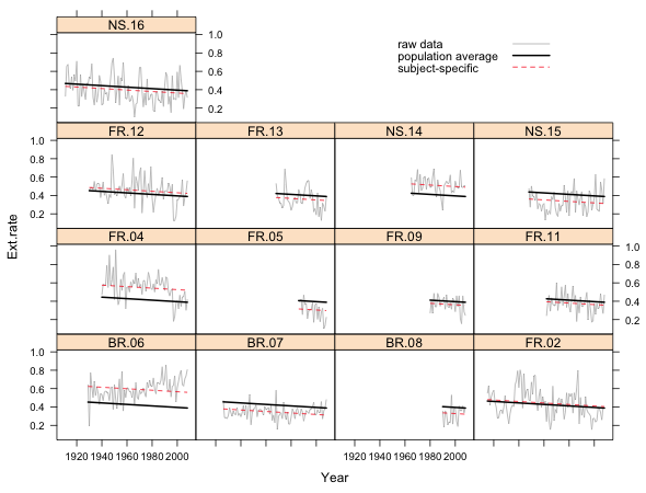
Fig. 1 Random intercepts model in separate panels
What we see in Fig. 1 are the raw data for each core connected by line segments, the subject-specific model, and the population average model. The population average model is exactly the same for each core but the subject-specific model varies from core to core. Because this is a random intercepts model, the subject-specific model differs from the population average model only in the value of its intercept. Thus all the displayed regression lines are parallel.
The variation of the actual observations about their individual subject-specific lines is the level-1 variance σ2. The variation of the individual subject-specific lines about the population average line is the level-2 variance τ2. Fig. 2 shows all the data and regression lines in a single figure and tries to distinguish the different roles that σ2 and τ2 have in the model.
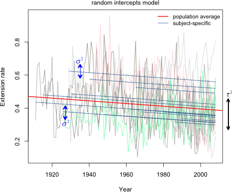
Fig. 2 Random intercepts model (R code)
While including random effects in a model induces a correlation structure in the response (see lecture 19), with long time series, like we have here, the induced correlation structure is typically inadequate. So, we should investigate whether the random intercepts model is properly accounting for the correlation. The method for checking this is to plot the ACF of the level-1 residuals.
Last week we used the acf function for this purpose, but to use it with grouped data we had to insert missing values between the residuals from the different groups to prevent observations from two different groups contributing to the correlations at the various lags. The nlme package has its own ACF function, ACF, that automatically accounts for the grouping that is specified when fitting an lme model. The ACF function assumes that the observations within a group are in their correct temporal order in the original data frame and that the time spacing of the observations is the same. If this is not the case, the results returned by ACF will not be sensible. The ACF function will also get the wrong answer if there are gaps in the time sequence. Because the observations in the coral cores data set are ordered correctly and there are no missing values we can use the ACF function here.
The ACF function acts on an lme model from which it extracts the level-1 residuals. To get a plot we use the output from ACF as the argument of the plot function. Confidence bands are displayed if a value for the alpha argument, the significance level for the bands, is given.
Because 20 lags are displayed we can modify the confidence bands with a Bonferroni correction that assumes that 20 tests have been carried out.
(a) 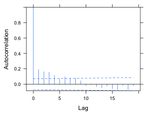 |
(b)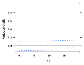 |
Fig. 3 ACF for the random intercepts model using (a) alpha = .05 and (b) alpha = .05/20, a Bonferroni correction to account for testing at 20 different lags. |
|
The displayed ACF has the signature of an autoregressive process. There is no PACF function in nlme so to produce one here we'd have to use the pacf function and go through the same protocol that we used in lecture 17. Because we already know a low-order ARMA process worked there, I just try fitting an AR(1) and ARMA(1,1) process and compare them using AIC. The syntax for including a correlation structure in an lme model is the same as it was for the gls function. We need to include a form argument in which we indicate the "time" variable and optionally a grouping term. Specifying the grouping structure is unnecessary here because we're updating a model and the group structure will be inherited from the model we're updating
The AIC indicates that the ARMA(1,1) model beats the AR(1) model and both beat a model with no correlation structure. To see if the correlation has been properly accounted for we can use the resType argument of ACF. Just like the type argument of residuals, resType can be used to tell ACF to extract normalized residuals. When we use the Bonferroni correction of Fig. 3b, both the AR(1) and ARMA(1,1) models appear to remove all the statistically significant correlations, but the correlation shows a much greater reduction with the ARMA(1,1) model.
(a)  |
(b)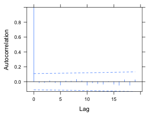 |
Fig. 4 ACF for the normalized residuals of a random intercepts model with (a) an AR(1) model for the residuals and (b) an ARMA(1,1) model for the residuals. An experimentwise α = .05 rate was obtained using a Bonferroni correction under the assumption that 20 lags were examined. |
|
If we compare the summary table of the model without a correlation structure to the model with an ARMA(1,1) model for the residuals we observe that there is a big difference in the standard errors and p-values.
Notice that the coefficient of Year has gone from being highly significant to being barely significant. The reason for that is simple. In model1 we treated the observations as being independent when they weren't. Because the observations are positively correlated the response variable exhibits much less variability than it should. When we account for this correlation we get a more honest estimate of the true variability of the response. Put another way, when we treat the observations as being independent we are exaggerating our sample size and hence our precision. When we properly account for the correlation the effective sample is much less than the naive sample size obtained assuming independence.
The random slopes and intercepts model adds a second equation at level 2 to the random intercepts model by allowing slopes to vary across cores. The multilevel model formulation is shown below.
where
The equivalent composite equation formulation, obtained by plugging the two level-2 equations into the level-1 equation, is shown next.
From this we can write down the R formulation of the model.
or equivalently
The summary output from this model does not look unusual but in fact there is a problem that manifests itself when we examine the variance components.
Notice that the variance of the random intercepts is reported to be 10–15, essentially zero, whereas in model1, the model without random slopes, it was estimated to be 0.007. What happened is that the lme function was not able to estimate both a random slope and a random intercept variance in this model. Usually the symptoms of this are more obvious than they are here, but the solution is the same—center the predictor. In multilevel models it is crucial that predictors in the model be roughly on the same scale. The magnitude of Year is currently too big. As we remarked in lecture 17 it's also the case that using a raw scale for Year is crazy because then the intercept corresponds to the extension rate in the year 0 A.D.
In a multilevel model centering is almost always necessary in order to obtain valid solutions. I refit the model centering year at 1967. Notice that centered year gets used in the random portion of the model too. This should be obvious because it is the coefficient of centered year, not year, that is being made random.
We now have obtained sensible results. The addition of random slopes has led to a large decrease in AIC. Notice that the variance components are also dramatically changed from the uncentered model.
From the output we see that ![]() = 0.00677,
= 0.00677, ![]() = 0.000002, and
= 0.000002, and ![]() = 0.0136. The reported correlation is the correlation between the random slopes and intercepts, which is now near zero.
= 0.0136. The reported correlation is the correlation between the random slopes and intercepts, which is now near zero.
The ranef function displays BLUPs of both the intercept and slope random effects.
The coef function adds these values to the corresponding fixed effects to obtain estimates of the random slopes and intercepts.
Fig. 5 displays the population average and subject-specific random slopes and intercepts models. As was the case in Fig. 1, the population-average line is the same in each panel but the subject-specific model varies. This time both the slopes and intercepts of these lines vary across panels.

Fig. 5 Random slopes and intercepts model in separate panels
Fig. 6 shows all the data and regression lines in a single figure and tries to distinguish the different roles the three variance components have in the model.
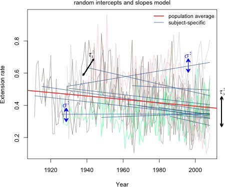
Fig. 6 Random slopes and intercepts model (R code)
It is possible to fit a model in which the slopes are random (each core gets its own slope) but the intercepts are fixed. To accomplish this we have to remove the intercept from the random formula with the -1 notation we've used previously. Thus we would need to write: random = ~I(Year-1967)-1|Core. When we compare the random slopes, random intercepts, and random slopes and intercepts models for these data, the random slopes and intercepts model has the lowest AIC.
The reef.type variable in the data set is a level-2 predictor because it varies only at the core level. It is a categorical variable with three levels so it needs to be converted to a factor when included in a regression model. By default R constructs the dummy variables alphabetically so that forereef and nearshore coral colonies are contrasted with backreef coral colonies.
Thus R has created two dummy variables of the following form.

To include reef.type in the model we have to decide in what way we think it alters the basic level-1 relationship between Ext.rate and centered Year. Does it modify the intercept, the slope, or both? The researchers hypothesized that it should modify the slope. We'll try all three possibilities.
If reef.type affects the intercept it should be entered into the level-2 equation for the intercept.
The corresponding composite equation is shown below. In it we see that reef type becomes part of the fixed effects portion of the model.
To estimate this model in R we start with the random slopes and intercepts formulation and just add reef.type to the fixed part of the model.
To see if reef.type affects the slope we enter it into the level-2 equation for the slope.
or in composite form
In R we specify this model by entering a term for the interaction between reef.type and I(Year-1967). Thus we need to include the term I(Year-1967):factor(reef.type) in the fixed part of the model expression.
If reef.type affects both the slope and intercept it should be entered into both of the level-2 equations.
or in composite form
From the composite form the fixed part of the model should include I(Year-19667), factor(reef.type) and the interaction between the two. We can obtain this in R as follows.
or using R's shortcut notation
where the * notation automatically generates all three terms (plus the intercept).
Based on AIC we should include reef.type as a predictor of the slopes but not the intercepts. Notice that in all three models the random portion of the model has remained the same. The random portion is determined by which coefficients in the level-1 model were declared to be random, not by predictors in the level-2 equations.
It may seem a little strange to consider a model with an interaction but without the corresponding main effect. Usually we would test the terms in model5 as follows.
These are variables added in order tests. The basic level-1 model appears on line 2. Line 3 tests whether the single population model should instead be three population models (based on reef type) that are parallel lines but with different intercepts. Based on the p-value the answer is no. When we add an interaction term so that the three population lines also have different slopes, we obtain a significant improvement (line 4).
In an ordinary regression model this is where we'd stop, but in a multilevel model removing the main effect of reef.type can make sense. Because this is a random slopes and intercepts model, individual cores already have different slopes and intercepts. So removing the reef type main effect does not lead to the silly constraint of forcing all the lines to pass through a single point. From the multilevel formulation it is clear that we can choose to add reef.type to the slope equation and not the intercept equation.
We can formally compare these models with a partial F-test because they're nested.
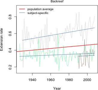
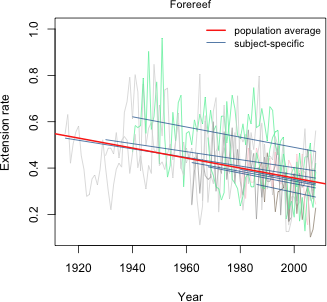
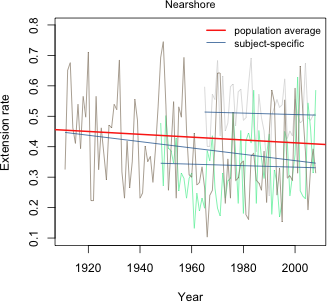
The non-significant result is consistent with our conclusions based on AIC. Allowing the population value of the intercepts to vary by reef type is not supported by the data. Fig. 7 displays the final reef type model, model4, as a panel graph. Unlike Figs. 1 and 5, now the population average model is not the same in each panel. Instead it varies by reef type.

Fig. 7 Random slopes and intercepts model with separate population slopes based on reef type
Fig. 8 displays this same model now divided into only three panels corresponding to the three different reef types. In each case the set of subject-specific lines in that panel varies randomly (i.e. the slopes and intercepts vary randomly) about the displayed population line.
 |
 |
 |
|
Fig. 8 Random slopes and intercepts model with separate population slopes based on reef type (R code)
A starting place when modeling hierarchical data is to first fit a variance components model, also called the unconditional means model. The variance components model is substantively uninteresting because it contains no predictors. It does however account for the structure in the data. Its value statistically is that it allows us to estimate variance components. In particular it allows us to determine how much variance lies within subjects versus how much variance lies between subjects. To allow for heterogeneity across level 2 units, it includes a random effect for each level 2 unit (core). The variance components model is the following.
where ![]() . To understand how the R specification of this model works, I substitute the level-2 equation into the level-1 equation to obtain the composite equation.
. To understand how the R specification of this model works, I substitute the level-2 equation into the level-1 equation to obtain the composite equation.
This last equation maps directly into R code as shown next.
Variance components are extracted from the model with the VarCorr function.
What's reported in the first column are the squares of the values reported in the summary table, so these are variances. From the output we determine that ![]() = 0.0077 and
= 0.0077 and ![]() = 0.0148. From this we learn a couple of things.
= 0.0148. From this we learn a couple of things.
We can use the output from VarCorr to calculate the intraclass correlation coefficient that was derived in lecture 19.
VarCorr has not produced a matrix, but a table, and the elements of the table are actually character values.
As a result our calculations of the correlation are rather awkward. I need to convert each character value to a numeric value before I can do arithmetic on it. (It's probably easier to just copy and paste the numbers.)
So the correlation between observations coming from the same core is 0.34, a modest value and far from 0. The implication is that the independence assumption of ordinary linear regression is not valid for these data.
The lme4 package is slated to eventually replace the nlme package. It extends normal mixed effects models to other members of the exponential family of distributions, thus permitting the fitting of generalized linear mixed effects models. Not all features are fully implemented so at the moment the nlme package has functionality not present in lme4. The lme4 package is not part of the standard installation of R, so it must first be downloaded from the CRAN site.
In lme4 the lmer function replaces lme. The major change in syntax is that there is no longer a random argument; the random effects are now written as part of the model formula. A second change is that to obtain maximum likelihood estimates one must specify the argument REML=FALSE.
Here are how some of the earlier lme models would be fit using lmer. The functions in the nlme package conflict with those inside lme4, so it's a good idea to first detach the nlme package before loading lme4.
A number of additional models are readily fit with the lmer function. For example, we can fit a random slopes and intercepts model in which the correlation of the two sets of random effects is constrained to be zero. Fitting such a model is rarely a good idea.
| Jack Weiss Phone: (919) 962-5930 E-Mail: jack_weiss@unc.edu Address: Curriculum for the Environment and Ecology, Box 3275, University of North Carolina, Chapel Hill, 27599 Copyright © 2012 Last Revised--February 26, 2012 URL: https://sakai.unc.edu/access/content/group/2842013b-58f5-4453-aa8d-3e01bacbfc3d/public/Ecol562_Spring2012/docs/lectures/lecture20.htm |