Lecture 19—Wednesday, February 22, 2012

Topics

• Random effects approach to dealing with observational heterogeneity
• Multilevel formulation of the random slopes and intercepts model
• The likelihood of a mixed effects model
  • Likelihood of the data at the cluster level
  • Joint distribution of the data and random effects
  • Obtaining the marginal likelihood of the data
  • Contrasting fixed and random coefficients
• The random intercepts model: a minimal model for correlated data

Random effects approach to dealing with observational heterogeneity

The random effects analog of the separate slopes and intercepts regression model is the random slopes and intercepts model.

with . In this model β₀ and β₁ represent the population-average coefficients while and are the deviations from this population average for coral core i. β₀ and β₁ can also be interpreted as the regression coefficients for a typical core, i.e., one corresponding to the middle of the distribution of random effects. The intercept for core i is and the slope is . Thus the random slopes and intercepts formulation of this model is also the following.

What makes this model different from the fixed effects model is that and are not directly estimated but instead are assumed to be drawn from a multivariate normal distribution.

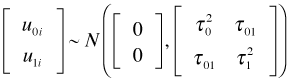
The diagonal entries of the multivariate normal covariance matrix are the individual variances of the intercept and slope random effects and the off-diagonal entry is their covariance. Because the correlation coefficient is defined by , an equivalent way of writing this distribution (and the one used by R) is the following.

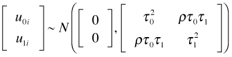
Rather than estimate the individual and we instead estimate the parameters of the covariance matrix of the multivariate normal distribution: ρ, τ₀, and τ₁. In the case of a normal response the likelihood simplifies in such a way that the individual and do not appear. For a non-normal response the random effects have to be numerically integrated out of the log-likelihood to yield what's called a marginal log-likelihood, which is then maximized.

The upstart is that in the random slopes and intercepts model we assume that the individual cores in the sample are drawn from a population of cores. The slopes and intercepts of individual cores are just typical random realizations from the population of slopes and intercepts from which they were drawn. Fig. 1 illustrates this situation for two specific cores that are numbered 1 and 2.

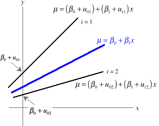
Fig. 1  Illustration of the random slopes and intercepts model

Multilevel formulation of the random slopes and intercepts model

It is common practice, particularly in sociology and political science, to formulate the random slopes and intercepts model slightly differently. Because it represents a hierarchy in the data, here annual rings nested in cores, it is convenient to write separate equations for each level of the hierarchy. These equations when combined yield the usual random slopes and intercepts model.

The level-1 model is a model for the individual rings contained within coral cores. Here, the level-1 model is just the trend model.

Level 1 model:, where , ,

The individual rings are called the level-1 units while the cores are called the level-2 units. The subscripts on the intercept and slope indicate that these parameters can potentially vary across cores, i.e., each core has its own separate regression equation. These equations define the level-2 model.

Level-2 Model: 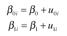where

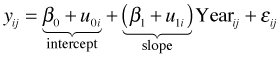
When we substitute the level-2 equations into the level-1 model we obtain the random slopes and intercepts model as before. In the multilevel formulation this combined expression is called the composite equation.

Composite equation:

The multilevel formulation is a great bookkeeping tool. In the coral core model variables that characterize individual annual rings, such as Year, appear in the level-1 equation. Year is a level-1 variable. Variables that characterize individual cores (and therefore all of the rings contained in that core) appear in the level-2 equations. Such variables are called level-2 variables. Notice that we have a choice of whether we enter a level-2 variable into the level-2 intercept equation, the level-2 slope equation, or both.

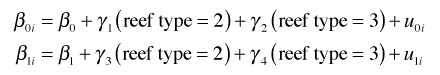
As an example suppose we decide to add reef type as a predictor in our model. Reef type is a characteristic of cores and hence is a level-2 predictor and should be added to the level-2 equations. It is also a categorical variable with three levels and hence will have to be added to the regression equation as two dummy variables. In the equations below I add it to both the intercept and the slope equation thus allowing both the intercept and slope to vary depending on the type of reef from which the core came.

Level 1 model:

Level-2 Model:

Now we have three population models, one for each reef type. The individual core regression lines in turn cluster about one of three population mean lines depending upon the reef type to which they belong. Fig. 2 illustrates this situation for two of the reef types, reef type 1 and reef type 2, and four cores, two from each reef type.

Fig. 2  Adding reef type as a level-2 predictor

From a modeling standpoint we would next test whether we need three population models (one for each reef type) to characterize the population of cores or just a single population model. Thus by using a mixed effects model we are able to include reef type in the model while at the same time letting each core have its own regression equation, something that was not possible in a purely fixed effects model.

The likelihood of a mixed effects model

Likelihood of the data at the cluster level

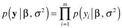
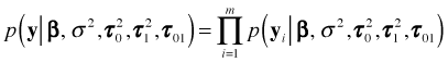
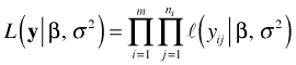
Methods employing maximum likelihood all start from the same point, the likelihood function. Recall that if we have a random sample of observations, , that are independent and identically distributed with probability density (mass) function where θ is potentially a vector of parameters of interest, then the likelihood of our sample is the product of the individual density functions. For the normal regression model θ will consist of the set of regression parameters β and the variance of the response σ², so that the likelihood can be written as follows.

With correlated data, i.e., structured data, the situation is more complicated. The data consist of observations where i indicates the level-2 unit and j the level-1 observation within that unit. Typically the level-2 units will be independent but the level-1 units will not be. If we let

so that , then we can write the likelihood in terms of the m clusters as follows where I include additional parameters that relate to the distribution of clusters.

Joint distribution of the data and random effects

If we choose to model the cluster structure using a mixed effects model then the are not the only random quantities to consider. The intercept and slope random effects also have a distribution. Thus the natural starting place in constructing the likelihood is with the joint density function of the data and random effects in cluster i, . From elementary probability theory we can write

• Here is the conditional distribution of the observed data assuming the values of the random effects are known. This will correspond to the probability model we assume for the data at level 1. For normal models this density will also be a function of the vector of fixed effect parameters β and the variance .
• is the joint distribution of the random effects. In all of the examples in this course this will assumed to be multivariate normal with mean zero and variance matrix that was given above.

Let . If we include the regression parameters in the likelihood then the joint distribution of the data and the random effects in cluster i would be written as follows

Conditional on the value of the random effects, the individual in cluster i are assumed to be independent. So we have

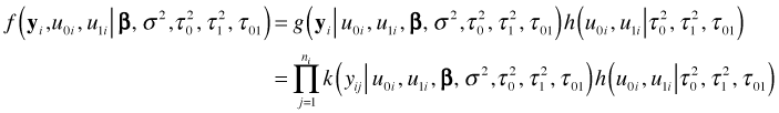
Here I use to denote the distribution of the individual conditional on the random effects and the regression and variance parameters.

Obtaining the marginal likelihood of the data

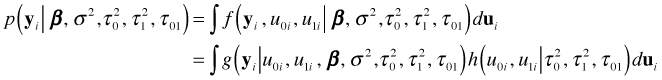
To go from a joint probability of , , and to a marginal probability for we integrate over the possible values of the random effects. Thus the marginal likelihood for cluster i is the following.

Putting all these pieces together we can write the marginal likelihood of our data as follows.

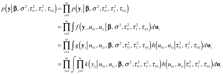
For the random intercepts model we've been considering the distribution of the random effects is normal and the distribution of the response given the random effects is normal. Thus both functions k and h in the last expression are normal densities. It turns out under this scenario that p is also a normal density and its mean and variance can be found from the means and variances of k and h. Thus with a normal model it is possible to find the marginal likelihood without doing the integration shown in the last expression. This is what the lme function of the nlme package does. For models in which k is not a normal distribution, e.g., binomial, Poisson or some other member of the exponential family, the integration needs to be carried out numerically in order to obtain the marginal likelihood. This is what the lmer function of the lme4 package does.

Contrasting fixed and random coefficients

It is worth comparing what the likelihood looks like for the separate slopes and intercepts model.

In this likelihood the vector β will also include the coefficients of the various dummy variables (now fixed effects) that are used to indicate group membership. These can then be used to obtain estimates of the slopes and intercepts of each group. So in the separate intercepts model we obtain estimates of all the group slopes and intercepts. In the random intercepts model we assume the intercepts arise from a common distribution and then estimate only the parameters of that distribution. If so then how can we get predictions of the intercept and slope random effects. How is this possible if the random effects are integrated out of the likelihood and are no longer present?

The predictions of the random effects are not obtained as a result of maximizing the likelihood. What happens is that after having estimated the regression parameters and variances in the marginal likelihood these estimates are used to obtain predictions of the random effects. Formally the predictions are the conditional means of the random effects distribution given the data and the regression parameters and are obtained using what amounts to a generalized least squares formula. The fact that they are the means of distributions gives them a distinct Bayesian flavor and they're sometimes called empirical Bayes estimates (also best linear unbiased predictors or BLUPs). So, unlike the separate slopes and intercepts model the steps taken to obtain predictions of the random slopes and intercepts are entirely post hoc.

The random intercepts model: a minimal model for correlated data

Fitting a random intercepts model is a minimal way to account for lack of independence in a hierarchical experimental design. Suppose we have a split plot design in which treatment A with two levels is randomly applied to groups (whole plots) and treatment B with two levels is random applied to individuals (split plots) separately within each group. The whole plots could be aquariums (with whole plot treatment "temperature") and the split plots could be individual fish in the tanks (with split plot treatment "species of fish").

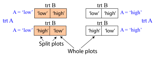
Fig. 3  Split plot design with whole plot treatment A and split plot treatment B

A minimal additive model that addresses the observational heterogeneity present in this design is the following random intercepts model (written in composite form).

where and and trtA and trtB are dummy variables indicating the treatment. (A more general model would allow also for an interaction between A and B but this is an unnecessary complication for the point I wish to make.)

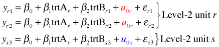
Consider the following three experimental units: two of them come from same group (level-2 unit r) and one comes from a different group (level-2 unit s). Here are their three regression equations.

Notice that both observations from level-2 unit r share the common random effect . The observation from level-2 unit s on the other hand possesses a different random effect, . The random effect then accounts for all those unmeasured characteristics that make group r different from any other group. Its presence causes members of this group to be similar to each other but different from members of other groups.

It can be shown that the random intercepts model induces a correlation in the observations coming from the same group. The relevant covariances are the following.

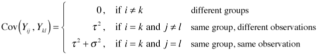
Observations from the same group (i = k) have a positive covariance, , while observations from different groups (i ≠ k) have a covariance of zero. So observations coming from the same group are more similar (have positive covariance) than observations coming from different groups (zero covariance).

Using the definition of correlation we can translate this statement about covariance into one about correlation. For distinct observations with j ≠ l we have

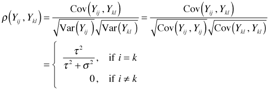
and so we see that observations coming from the same level-2 unit (group) are correlated while observations from different level-2 units are uncorrelated.

Observe that the correlation structure is really very simple. Any two observations from the same level-2 unit have the same correlation. If we let 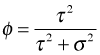then the correlation matrix for any level-2 unit takes the following form.

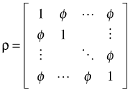
Such a constant correlation matrix is called exchangeable. If we assemble these exchangeable correlation matrices ρ for all the level-2 units into a single matrix in which all observations are represented we obtain the following block-diagonal correlation structure for the model.

where each ρ_i is an exchangeable correlation matrix like the one shown above and 0 is a matrix of zeros.

Course Home Page