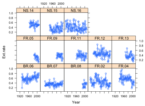
Fig. 1 Panel graph of the extension rate time series in which each panel represents the data from a different core
Here's a description of today's data set taken from the abstract of Castillo et al. (2011).
Natural and anthropogenic stressors are predicted to have increasingly negative impacts on coral reefs. Understanding how these environmental stressors have impacted coral skeletal growth should improve our ability to predict how they may affect coral reefs in the future. We investigated century-scale variations in skeletal extension for the slow-growing massive scleractinian coral Siderastrea siderea inhabiting the forereef, backreef, and nearshore reefs of the Mesoamerican Barrier Reef System (MBRS) in the western Caribbean Sea. Thirteen S. siderea cores were extracted, slabbed, and X-rayed. Annual skeletal extension was estimated from adjacent low-and high-density growth bands.
The data we have are the annual extension rates (the amount a coral colony grows in a year) from 13 different samples. Cross-sections of cores taken from coral colonies exhibit rings much like tree trunks do. I load the data from the class web site that I previously downloaded to my laptop and examine the first few observations.
Each column contains the record from a different coral core. The first part of the variable name identifies the reef type (FR = forereef, BR = backreef, NS = nearshore) and the second part the sample number. The sample labeled FR.10 has all missing values, NA. It was discarded after it was discovered that the growth bands were too distorted to provide reliable readings.
There are some issues with the data file. Each coral core provides a different amount of data with some colonies being older than others. When this happens missing values were entered for the earlier years going all the way back to 1900. In truth none of the cores have data going back this far so that a number of years have missing values for all the samples. The earliest dated band corresponds to 1911 as we can see in the output below.
More alarming is the fact that the end of the file contains rows of all missing values, even for Year!
What we're seeing here is a "feature" of Excel that has been present for over a decade. When files are exported from Excel as comma-delimited text files, Excel will often append extra blank rows at the end of the file consisting of commas but no data. This has occurred in this file so we'll need to eliminate these spurious rows of "data".
The goal of this lab session is to model the extension rates over time to determine if the reef location, (FR, BR, or NS), has an effect. In doing so we will need to respect the structure of the data, the fact that observations are nested in cores. This isn't a random sample of extension rates, instead we have a random sample of cores from which were then obtained all the annual extension rates. So, although observations from different cores are probably independent, it's unlikely that the observations coming the same core are. Put another way the data here are heterogeneous. We have observations coming from different cores as well as multiple observations coming from the same core. Furthermore, because the growth rings were measured over time we might expect measurements made in successive years to be more similar to each other than they are to measurements made far in the past. Thus we will need to examine the residuals of our regression models for evidence of lingering temporal correlation.
The set-up of the current data frame is not appropriate for fitting regression models. Annual extension rate is the response so it needs to appear as a single column not scattered across 14 different columns as is currently the case. We will need to stack these columns keeping track of the years represented by the individual elements. We'll also need to create new variables that identify the core from which the observations came as well as the reef type for that core.
The first task is to stack into a single column the columns of the data frame that contain the extension rates. The unlist function will do this (because technically the columns of a data frame are the elements of a list).
Next we need to repeat the entire Year column once for each of the 14 columns we're unlisting. This can be accomplished with the rep function. The rep function can be used in two distinct ways.
The following simple examples illustrate these two uses of rep.
The repeated Year variable is created with rep using the first method.
The Core labels currently are the column names in the original data frame. A variable that identifies the Core can be created with rep using the second method. Because the number of rows of the data frame we're unlisting is nrow(ext.temp) = 141, the second argument of rep should be a vector containing the number 141 repeated 14 times. We can generate this efficiently by using a rep call as the second argument of rep.
To assemble the results in a new data frame, I use the data.frame function and then assign names to the newly created columns.
Next we create a reef type variable. The first two letters of the Core name identify the reef type. I use the subset function of R to extract these two letters. Here substr(ext.rates.temp$Core,1,2) extracts the letters of Core that begin at position 1 and end at position 2.
The missing values in the data set are all superfluous. None of them are there to denote gaps in a time series. Therefore it is safe to remove them. To remove the missing values I use the is.na function. is.na(x) evaluates to TRUE if x is missing, and FALSE if not. Therefore when preceded by !, R's logical not symbol, !is.na(x) is TRUE if x is not missing. I use it as a row condition to extract only the non-missing observations in the data frame.
Because the data come to us in units, cores, it is important when displaying the data graphically that this structure is preserved. The xyplot function of the lattice graphics system is designed to generate such plots. I begin by sorting the data by Year separately for each core.
The basic syntax is xyplot(y~x|z) where z is the grouping variable. What's displayed is the relationship y~x separately for each distinct value of z. The variable z is a conditioning variable such that each distinct value of z will correspond to a separate panel in the displayed output.
Because this is a time series we should connect consecutive points with line segments. To display both points and lines I include the argument type='o' where 'o' signifies overlay.
|
Fig. 1 Panel graph of the extension rate time series in which each panel represents the data from a different core |
From the graph it appears there may be an increasing trend in the backreef cores and perhaps a negative trend in some of the forereef cores.
I start by fitting a sequence of models that ignores the structured nature of the data. I fit in order
To obtain more meaningful estimates I elect to center the predictor Year. Centering means subtracting off a fixed constant from the predictor. In an uncentered model, y~x, the intercept estimates the mean response when x = 0. For the current data set this would correspond to the mean annual extension rate in the year 0 AD, an absolutely useless (and nonsensical) piece of information. Instead, I center the variable Year so that the intercept corresponds to the mean for a year that actually occurs within the range of the data. For various reasons I choose the year 1967 as the centering constant. The centering can be done by creating a new variable in the data frame, or it can be done on the fly within the regression equation by using the I function as follows: lm(Ext.rate~I(Year-1967), data=ext.rates2). The I function causes the arithmetic specified in its argument to be performed before the regression model is fit. In this case, 1967 is subtracted from the value of Year for each observation. The slopes of the centered and uncentered models are exactly the same; only the intercepts are different.
The results indicate that it is necessary for each core to have its own intercept. The closeness in the AIC of the last two models suggests that the evidence for requiring each core to have a separate slope is not as strong as it is for the intercepts. I carry out a formal partial-F test to verify this.
Model 1: Ext.rate ~ I(Year - 1967) + factor(reef.type):I(Year - 1967) +
factor(Core)
Model 2: Ext.rate ~ I(Year - 1967) + factor(Core):I(Year - 1967) + factor(Core)
Res.Df RSS Df Sum of Sq F Pr(>F)
1 751 10.3648
2 741 10.0581 10 0.3068 2.2599 0.01328 *
---
Signif. codes: 0 ‘***’ 0.001 ‘**’ 0.01 ‘*’ 0.05 ‘.’ 0.1 ‘ ’ 1
The significance test agrees with AIC suggesting that each core is sufficiently different that it needs a separate slope and intercept. The reef type pattern is not able to adequately account for individual core differences. Of course all of these results are tentative because we've not yet addressed the temporal correlation that may be present in the data.
Because the data were recorded over time we might expect later values to be influenced by earlier values. The predictors in our model may have accounted for some of the original temporal correlation in the data, so we should examine the residuals of the model. The temporal correlation if it exists should be present within a core not between cores, thus we have 13 separate time series to look at. It would be desirable to use the data from all cores simultaneously to obtain a better estimate of the correlation. The acf function we will use to examine the autocorrelation function (ACF) uses the relative position of the values in a vector to determine their separation in time. Thus we can't simply concatenate the different time series because this would mess up the calculation of lags. The last year of one series would be adjacent to the first year of the next series and the values from these different series would incorrectly contribute to the short-term lag correlations. The trick to doing this correctly is to introduce missing values between each core series before stringing together the residuals from the separate cores as one long time series. Enough missing values should be used to prevent cross-core contamination at the temporal lags of interest.
I first use the split function to divide the residuals into separate groups based on the core from which they came. The split function creates a list because the residual vectors from different cores are of different lengths. We've previously accessed the components of lists with the $ notation, but lists can also be accessed numerically by their position using the double subscript notation, [[ ]]. I use a for loop indexed by i to repeatedly carry out a sequence of operations for different values of the index i. Each time through the loop a vector of residuals from a different core is selected to which 30 missing values are then appended. This new vector is then added to the growing vector of residuals and missing values generated up until this point.
The R acf function has an argument na.action=na.pass that causes it to skip over the missing values (while still keeping track of the time differences). I also include the lag.max=30 argument so that only 30 lags are displayed. Because only 30 missing values were inserted between the time series, at lags greater than 30 the residuals from one core will be contaminated with those from the next core. I use the ci argument to set a 95% confidence band with a Bonferroni correction to account for the fact that we'll be carrying out 30 tests of significance at 30 different lags.
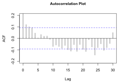 |
Fig. 2 Plot of autocorrelation function of the residuals |
The plot shows a few significant correlations at early lags and then a number of additional significant correlations beginning at around lag 15. Unfortunately, the displayed confidence bounds are incorrect. The acf function is using the “wrong” fixed sample size. It is counting the NAs. We can see this by assigning the results of the acf function to an object and examining the $n.used component.
To correct this we need to add the confidence bounds ourselves using the correct sample sizes for each lag. The formula for the error bounds of the ACF is

Here L is the total number of lags being tested,![]() is a quantile of a standard normal distribution, and N(k) is the number of observations available at lag k. As an illustration of determining N(k) I compute the number of observations available for calculating the lag 30 correlation. To obtain the numbers of observations in each core I use the table function.
is a quantile of a standard normal distribution, and N(k) is the number of observations available at lag k. As an illustration of determining N(k) I compute the number of observations available for calculating the lag 30 correlation. To obtain the numbers of observations in each core I use the table function.
The number of pairs of observations a distance 30 years apart is obtained by subtracting 30 from these values.
The negative values can be removed by multiplying them by a Boolean condition that tests if the calculated values are positive or not.
Finally we sum these up.
To carry out these calculations at each lag, I write a function in which I replace 30 in the above expression with a variable and then sapply the function to the numbers 0 through 30, the possible lags.
I now use these values in the formula for the confidence bands given above and draw my own bands. It is not possible to turn off the display of the default confidence bands from the acf function, so I just color them white using the ci.col argument. (A better solution is to draw the spikes ourselves.)
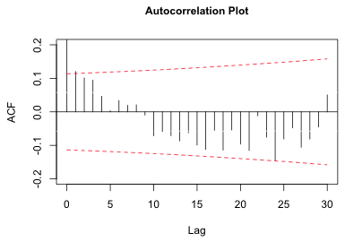 |
Fig. 3 Plot of autocorrelation function for the residuals |
While the picture has improved, there is still a significant correlation at lag one, and perhaps another at lag 24. The Bonferroni correction guarantees that no more than 5% of the observed significant lags are due to chance. With 30 lags that comes to 1.5 spurious significant results. Given that there are possibly two significant lags in Fig. 3, with one at lag 1, we probably shouldn't attribute them to chance.
While the ARMA models we discussed last time can be used to remove residual correlation at low lags, they are rather ineffectual at dealing with periodic behavior. The pattern in Fig. 3 looks distinctly sinusoidal suggesting that adding a trigonometric term to the regression model might eliminate the observed periodic pattern. The graph suggests that a sine function with a period of 40 years might work, but we should use the data to estimate the amplitude, period, and phase angle. We can accomplish this by fitting the following model with a value specified for k.
update(model4, .~.+cos(2*pi/k*Year)+sin(2*pi/k*Year))If we specify the value for k, the period, R will estimate coefficients b1 and b2 for the cosine and sine. Using a little trigonometry we can rewrite the sum of a cosine and sine of the same angle as follows.
In the second line I noticed that the coefficients of the original cosine and sine are clearly the sine and cosine of some angle that I call φ. (Proof: the two coefficients lie between –1 and 1 and if you square them they sum to 1.) In the last line I use the sine of the sum of two angles identity where the angles are ![]() and φ. So by adding the sine and cosine term to the regression model we are actually adding a single sine function with amplitude A, period k, and phase angle φ.
and φ. So by adding the sine and cosine term to the regression model we are actually adding a single sine function with amplitude A, period k, and phase angle φ.
The estimated regression equation will provide values for A and φ, but we still need to specify k. To obtain the maximum likelihood estimate of k, I set up a profile likelihood problem. I fit the model for a range of plausible integer values for k, examine the AICs (or log-likelihoods) of the resulting models, and select the model that yields the smallest AIC (largest log-likelihood).
The code below estimates a model with a periodic term in which the period k ranges from 1 to 60. I begin by creating a variable to store the results, a matrix with 2 columns and 60 rows that I populate initially with missing values. I then fit the model for various values of k each time computing the AIC and storing it in the matrix along with the corresponding value of k.
I use the which.min function to determine the position of the smallest AIC value in the matrix of results.
So we need a sine function with a period of 36 years. It might be interesting to plot the AIC values to see if this choice is unambiguous.
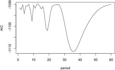 |
Fig. 4 Plot of AIC for different choices of the period of the periodic function |
With this choice for the period, we can refit the regression model with a periodic term, extract the residuals, and examine the autocorrelation function again.
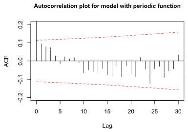 |
Fig. 5 Autocorrelation plot of the residuals for a model with a periodic function |
The significant long-range correlations have been removed as have the short-range ones.
Although the lag 24 correlation in Fig. 3 was at best marginally significant, the lag 1 correlation was definitely significant. Rather than try to model the periodicity we could instead focus on the significant lag 1 residual correlation in model4 and treat the apparent periodicity as spurious. The short-term correlation pattern displayed in Fig. 3 shows an exponential decay with increasing lag. This is usually the signature of an autoregressive process. As was explained in lecture 16, the partial autocorrelation function can be used to determine the order of the autoregressive process. If we plot the partial autocorrelation function for model4 using the pacf function of R we obtain the following.
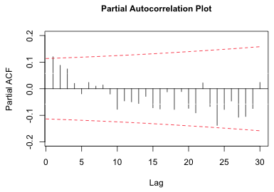 |
| Fig. 6 Partial autocorrelation plot of the residuals |
There is only one significant lag in the PACF suggesting that perhaps an AR(1) process is appropriate. Because the PACF is decaying exponentially and not dropping off suddenly to zero, some mixture of an autoregressive and moving average process might be a better choice. In any case it is pretty clear that an ARMA(p,q) process with fairly low values for p and q, perhaps no more than 1, will suffice.
As was discussed in lecture 15, correlation structures for the residuals can be added to an ordinary regression model by using generalized least squares. The gls function in the nlme package implements generalized least squares. To specify a correlation structure the correlation argument of gls is included in which one of the standard classes of correlation structures (corStruct) available in the nlme package is used. For instance, to specify an ARMA(1,1) model that is fit separately to each core using centered Year as the time variable we would write the following:
correlation=corARMA(p=1, q=1, form = ~ I(Year-1967) | Core)
The form argument of corARMA identifies the variable that records time in the model, I(Year-1967) in our case, and a grouping variable if there is one, which is Core here. Just as with the xyplot function of lattice, a vertical bar is used to separate the time variable from the grouping variable. The gls function provides a couple of different methods for estimating the ARMA parameters of which maximum likelihood is one. Because we want to compare models using AIC we need to tell gls to use maximum likelihood by including the argument method='ML'.
I next fit a sequence of ARMA(p,q) models using different values of p and q and then compare the models obtained to the original model using AIC. In order to keep track of the results, I set this up as two nested loops that cycle through different values of p and q. I have to exclude the possibility of p = 0 and q = 0 explicitly with an if conditional programming statement because this is not a legal combination in the corARMA function. The notation p>0 | q>0 causes the statements that follow it to be executed only when at least one of p or q is not zero. Although it is purely overkill here, I try fitting all possible ARMA(p,q) processes up to order 3. I store the results in an object called cor.results that is initialized to NULL (meaning empty). Each new vector of results is then added to this object by attaching them at the end with the rbind function.
Error in gls(Ext.rate ~ I(Year - 1967) + factor(Core):I(Year - 1967) + :
function evaluation limit reached without convergence (9)
The error message indicates that one of the models failed to converge. Because we were saving the results incrementally we can examine the results so far to see where things went wrong.
The first missing model is the ARMA(2,3) model. So either it failed to converge or the last reported model, ARMA(2,2), failed to converge. Because this is way past what we think is a reasonable model anyway, I skip over it. I restart the loop with p = 3 and try to finish the rest of the models.
p q logLik AIC
[1,] 0 1 578.5313 -1101.063
[2,] 0 2 580.9363 -1103.873
[3,] 0 3 583.6040 -1107.208
[4,] 1 0 579.3271 -1102.654
[5,] 1 1 583.5647 -1109.129
[6,] 1 2 582.0690 -1104.138
[7,] 1 3 583.8434 -1105.687
[8,] 2 0 582.1162 -1106.232
[9,] 2 1 583.7883 -1107.577
[10,] 2 2 612.9906 -1163.981
[12,] 3 0 584.0702 -1108.140
[13,] 3 1 584.1622 -1106.324
[14,] 3 2 584.1936 -1104.387
[15,] 3 3 584.9909 -1103.982
[16,] 0 0 573.8058 -1093.612
If the output is to believed, an ARMA(2,2) model is the clear winner followed by an ARMA(1,1) model as a distant second. The fact that a mixed autoregressive and moving average process ranks best is consistent with what the ACF and PACF plots revealed. The fact that it is an ARMA(2,2) process is a bit surprising. But if we scrutinize the results from the other models it becomes quite clear that the log-likelihood reported for the ARMA(2,2) process is wrong.
How do we know this? When we examine a sequence of nested models the value of the log-likelihood must be a monotone increasing function of the number of parameters. Adding a parameter to a previously estimated model cannot cause the log-likelihood to decrease. At worst the log-likelihood may stay the same if the new parameter contributes nothing to the model. Not counting the correlation parameters of the ARMA(p,q) process, each model estimates 27 parameters. If we focus on two different sequences of nested models that sandwich the ARMA(2,2) model we see that there is a problem.
Model |
p |
q |
logLik |
# parms |
Model |
p |
q |
logLik |
# parms |
ARMA(2,1) |
2 |
1 |
583.7883 |
30 |
ARMA(1,2) |
1 |
2 |
582.0690 |
30 |
ARMA(2,2) |
2 |
2 |
612.9906 |
31 |
ARMA(2,2) |
2 |
2 |
612.9906 |
31 |
ARMA(2,3) |
2 |
3 |
NA |
32 |
ARMA(3,2) |
3 |
2 |
584.1936 |
32 |
Based on the two nested sequences of models that are shown, it is clear that the correct log-likelihood of the ARMA(2,2) model must lie between 583.79 and 584.19. The reported value of 612.99 has to be wrong.
Discarding the ARMA(2,2) model results as being spurious, the model with the lowest AIC is an ARMA(1,1) model.
The ARMA(1,1) model for the residuals is
![]()
where ![]() and φ1, θ1, and σ2 are parameters that are estimated by gls.
and φ1, θ1, and σ2 are parameters that are estimated by gls.
When we specify a correlation model for the residuals, we don't remove the correlation , we attempt to model it. Thus an ACF of the ordinary residuals will still the resemble Fig. 3. To determine if the choice of correlation model is correct we can plot the ACF of the normalized residuals from our model. According to the help screen of residuals.gls, specifying type = "normalized" as an argument to the residuals function yields standardized residuals that are pre-multiplied by the inverse square-root factor of the estimated error correlation matrix. If the specified correlation model is correct, the ACF of the normalized residuals should no longer show a significant pattern. I extract the normalized residuals, insert missing values between the core time series, and plot the ACF.
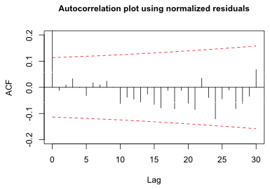 |
| Fig. 7 ACF of the normalized residuals from an AR(1,1) model |
The plot reveals that the significant lag 1 correlation has been removed. The previously observed periodic behavior has also been removed.
Recall that the point of accounting for correlation was to ensure that we can draw valid conclusions when using AIC and/or significance testing for model selection. Previously we concluded that the best model was one that allowed each individual core to have its own intercept and slope. That conclusion must now be changed. I refit model3 with an ARMA(1,1) correlation structure for the residuals and compare it to model4 with the same correlation structure.
The two models are not significantly different. Now the best model is the simpler one in which in the intercepts are different for each core, but the slopes vary by reef type. This confirms the researchers' hypothesis that the trend over time has been different depending upon the environment of the coral colony. Colonies in the nearshore and forereef environments have an annual extension rate trend that is less than that of reefs in the backreef environment. The backreef colonies exhibit a weak positive trend while those in the nearshore and forereef environments exhibit a negative trend. Of these only the trend in the forereef is significantly different from zero (details not shown).
| Jack Weiss Phone: (919) 962-5930 E-Mail: jack_weiss@unc.edu Address: Curriculum for the Environment and Ecology, Box 3275, University of North Carolina, Chapel Hill, 27599 Copyright © 2012 Last Revised--February 19, 2012 URL: https://sakai.unc.edu/access/content/group/2842013b-58f5-4453-aa8d-3e01bacbfc3d/public/Ecol562_Spring2012/docs/lectures/lecture17.htm |