The autocorrelation function is usually examined graphically by plotting ![]() against
against ![]() in the form of a spike plot and then superimposing 95% (or Bonferroni-adjusted 95%) confidence bands. We expect with temporally ordered data that the correlation will decrease with increasing lag. Fig. 1 shows a plot of the ACF that is typically seen with temporally correlated data. Here the correlation decreases exponentially with lag.
in the form of a spike plot and then superimposing 95% (or Bonferroni-adjusted 95%) confidence bands. We expect with temporally ordered data that the correlation will decrease with increasing lag. Fig. 1 shows a plot of the ACF that is typically seen with temporally correlated data. Here the correlation decreases exponentially with lag.

Fig. 1 Display of an ACF with 95% confidence bands
The confidence bands for the ACF are calculated using the following formula.

Here z(p) denotes the quantile of a standard normal distribution such that P(Z ≤ z(p)) = p. For an ordinary 95% confidence band we would set α* = .05. For a Bonferroni-corrected confidence bound in which we attempt to account for carrying out ten significance tests (corresponding to the ten nonzero lags shown in Fig. 1) we would use α* = .05/10. We examine the rationale for this correction in the next section.
The multiple testing problem deals with the probability of falsely rejecting the null hypothesis when a collection of tests are considered together. It stems from the simple observation, developed more fully below, that the more tests you do the more likely it is that you'll obtain a significant result by chance alone. The "problem" is deciding whether anything should be done about it. This is a surprisingly contentious issue.
Consider again the situation shown in Fig. 1. The displayed residual correlations at ten different lags along with the 95% confidence bands allow us to carry out ten individual tests. At each lag if a spike pokes beyond the confidence band, we would declare the correlation at that lag to be significantly different from zero at α = .05. Remember that α = Prob(Type I error) = P(reject H0 when in fact H0 is true). So given that we have a 5% chance of making a Type I error on each of the ten tests individually, what's the probability that we make at least one Type I error in doing all ten of these tests? This is called the experimentwise (or familywise) Type I error. We set the individual α-levels at some fixed value, say α = .05, and are now concerned how that translates into an experimentwise α-level when we consider all the individual tests together.
It's easy to derive a formula for experimentwise error.
The last expression involves calculating the probability of the intersection of ten simple events. Recall that in general ![]() .
So we have three scenarios to consider:
.
So we have three scenarios to consider:
chocies.gif)
Because the same residuals contribute to each of the different lag calculations we would expect the ten simple events in the intersection to be positively correlated with each other. Rather than try to estimate this correlation we'll instead assume the events are independent (scenario 1). Because the events are actually positively correlated (scenario 2), making this assumption will cause us to underestimate the joint probability above which in turn means we will overestimate the probability of making at least one Type I error. As a result the formula we obtain assuming independence is actually a worst-case scenario. Bender and Lange (2001) refer to this as the maximum experimentwise error rate (MEER).
So we have, assuming independence
But we've set the probability of a Type I error equal to α in each of these tests. So each of these probabilities is 1 – α. Thus we have
If we carry out n tests the experimentwise error becomes
![]()
Using R we can estimate how large this probability becomes for fixed α when n is allowed to vary.
So by the time we've done 15 tests there's at least a 50-50 chance that we've made a Type I error somewhere in the process. So, what should we do? There are two basic options:
Adjusting α is a reasonable choice, but it comes at a cost. There is an inverse relationship between α and β, the Type I and Type II errors. If we decrease α on each test we necessarily increase β. Fig. 2 illustrates the tradeoff between α and β for a simple one-sample hypothesis test. The distance d that is shown between the two distributions represents a difference that is considered biologically important. The old α (solid pink) and the old β (solid green) represent the original Type I and Type II errors. When α is decreased to new α (α* = red hatched region only), the old β is increased so that it now also includes the region labeled "increase in β" (β* = green hatched region plus solid green region).
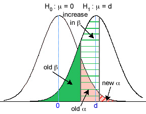
Fig. 2 Type I and Type II errors in a two-sample hypothesis test
Hence controlling the experimentwise Type I error inflates the individual Type II errors. Since power = 1 – β, another way of saying this is that controlling the experimentwise Type I error leads to a loss of power for detecting differences in each of the individual tests. This strategy is considered acceptable largely because it is so difficult to quantify the Type II error given that it depends on the true, but unknown, state of nature.Let
![]() = α-level for individual tests and let
= α-level for individual tests and let ![]() = experimentwise α-level. Our goal is to choose
= experimentwise α-level. Our goal is to choose ![]() in order to achieve a desired
in order to achieve a desired ![]() as given by the experimentwise error formula
as given by the experimentwise error formula
![]()
The Dunn-Sidak method makes the following choice for ![]() .
.
![]()
The simplest way to see that the Dunn-Sidak method works
is to plug this choice for ![]() into the experimentwise error formula above.
into the experimentwise error formula above.
which is what we want. The R function below carries out the Dunn-Sidak calculation. We illustrate its use in a scenario where there are 10 tests and we desire the experimentwise Type I error rate to be .05.
The Dunn-Sidak formula suggests
that ![]() , the α-level used for each individual test, should be almost
a factor of 10 smaller, .0051, than the desired experimentwise α.
, the α-level used for each individual test, should be almost
a factor of 10 smaller, .0051, than the desired experimentwise α.
The Bonferroni procedure is a linear approximation to the Dunn-Sidak formula. It owes its popularity to the fact that it is trivial to calculate. Calculus provides us with the formula for the binomial series, a generalization of the binomial theorem to exponents other than positive integers. Unlike the binomial formula, the binomial series expansion involves an infinite number of terms.
Since 0 < α < 1, we can use the binomial series
formula with x = –α and ![]() to obtain a series expansion of the
to obtain a series expansion of the ![]() term that appears in the Dunn-Sidak formula.
term that appears in the Dunn-Sidak formula.
where in the last step all terms are dropped except for the first two. The error in this approximation can be determined from the error formula for a Taylor series. In particular, with x = –α the above series is an alternating series, so the truncation error turns out to be no greater than the magnitude of the first term omitted. Since the first omitted term squares α and divides by n2, the error of this approximation will be small. Plugging this approximation into the Dunn-Sidak formula yields the Bonferroni criterion for the α to use on individual tests.
For the scenario we've been considering, 10 tests and a desired experimentwise Type I error of .05, the Bonferroni criterion yields: .05/10 = .005. This is hardly different from the recommendation of the Dunn-Sidak method.
Another diagnostic that is useful in certain circumstances is the partial autocorrelation function (PACF). Suppose we regress each residual against the first k lagged residuals as in the following regression equation.
![]()
The coefficient βk in this regression is called the partial autocorrelation at lag k. It represents the relationship of a residual to the residual at the kth lag after having removed the effect of the residuals at lags 1, 2, …, through k – 1. After we plot the ACF, depending on what it shows, a plot of the PACF at lag k versus k can be helpful in choosing an appropriate correlation model for the residuals. Further details are given below.
Typically the ACF and PACF are used jointly to identify an appropriate ARMA correlation model for the residuals. For an ARMA model to be appropriate the observations need to be equally spaced in time. (This caveat also holds for the use of the ACF.)
A residual autoregressive process is defined by a recurrence relation that expresses the residual at a given time as a linear function of earlier residuals plus a random noise term. In an autoregressive process of order p, the residuals are related to each other by the following equation.
![]() ,
, ![]()
where φ1, φ2, … , φp are the autoregressive parameters of the process. In an autoregressive process a residual is affected by all residuals p time units or less in the past. The term at represents random noise and is uncorrelated with earlier residuals.
The various φ coefficients in this model are difficult to interpret except in the simplest case of an AR(1) process. For an AR(1) process we have
![]()
for t = 2, 3, … and ![]() . If we write down the equations for the first few terms and carry out back-substitution we get the following.
. If we write down the equations for the first few terms and carry out back-substitution we get the following.
Because the noise terms are uncorrelated we find that for any time t,
![]()
So for an AR(1) process the correlation decreases exponentially over time by a factor φ. For other autoregressive processes the correlation at various lags is much more complicated, but it is still the case that the ACF of all autoregressive processes decreases in magnitude with increasing lag.
A residual moving average process is defined by a recurrence relation that expresses the residual at a given time as a linear function of earlier noise terms plus its own unique random noise term. In a moving average process of order q, the residuals are related to each other by the following equation.
![]()
where θ1, θ2, … , θq are the moving average parameters of the process. The simplest example is an MA(1) process which is defined by the recurrence relation
![]()
for t = 2, 3, … and ![]() . The parameter θ has no simple interpretation. Generally speaking moving average processes provide good models of short term correlation.
. The parameter θ has no simple interpretation. Generally speaking moving average processes provide good models of short term correlation.
An ARMA(p, q) process, autoregressive moving average process of order p and q, is a process includes both an autoregressive component and a moving average component. The parameter p refers to the order of the autoregressive process and q is the order of the moving average process. The general recurrence relation for a residual ARMA(p, q) process is the following.
![]()
where φ1, φ2, … , φp are the autoregressive parameters of the process and θ1, θ2, … , θq are the moving average parameters of the process.
One strategy for choosing a residual temporal correlation structure is to fit a number of different ARMA(p, q) models using maximum likelihood and then choose the correlation structure that yields the largest decrease in AIC. The problem with this approach is that there are too many models to consider and we may end up capitalizing on chance in selecting a best model.
A more parsimonious approach is to use diagnostic graphical techniques to narrow the search down to a smaller set of candidate models. For instance, if graphical diagnostics suggest an AR(2) model might be an appropriate choice, we might also try fitting an AR(1), AR(3), MA(1), MA(2), ARMA(1,1), and perhaps a few other processes for the residuals and then choose the best among these using AIC. If a number of models turn out to be equally competitive I would defer to the graphical results in selecting the final model. In what follows I describe the graphical signatures of various ARMA processes.
| Pattern | Conclusion |
| ACF decaying exponentially to zero (alternating or not). | AR process. The number of significant lags in the PACF determines the order of the process. |
In an autoregressive process the magnitude of the correlation decreases exponentially with increasing lag. If, e.g., one or more of the autoregressive parameters are negative, the correlations can change sign at different lags but their magnitudes will still decrease exponentially. For an autoregressive process of order p, a plot of the PACF will show p significant lags after which the PACF drops precipitously to near zero. Fig. 3 shows the ACF and PACF of an AR(1) process with φ = 0.8 . Observe that only the first lag of the PACF is statistically significant corresponding to p = 1.
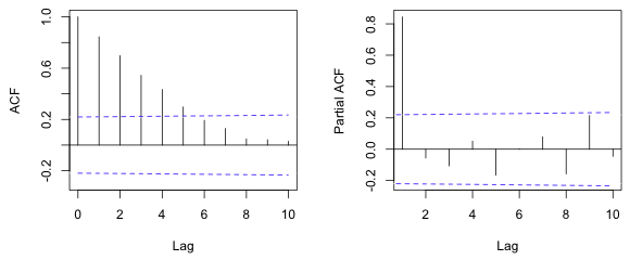
Fig. 3 ACF and PACF of an AR(1) process (R code)
| Pattern | Conclusion |
| ACF with one or more significant spikes. The rest of the spikes are near zero. The PACF decays exponentially to zero. | MA process. The number of significant spikes in the ACF determines the order of the process. |
In a moving average process the number of consecutive significant spikes in the ACF identifies the order of the process, after which the correlation is zero. (Compare this to the autoregressive process described above.) Often the PACF will show an exponential decay in the magnitudes of the spikes at consecutive lags. As an illustration Fig. 4 shows the ACF and PACF of an MA(2) process with θ1 = 3 and θ2 = 2 . Observe that the first two lags of the ACF are significant, q = 2, and the PACF shows oscillatory decay to zero.
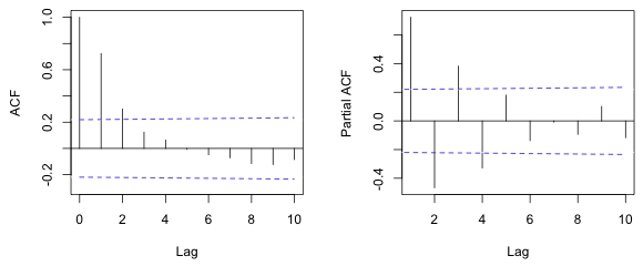
Fig. 4 ACF and PACF of an MA(2) process (R code)
| Pattern | Conclusion |
| ACF exhibits a few significant spikes followed by a decay. The ACF and PACF are hybrids of the AR(p) and MA(q) patterns. | ARMA(p, q) process. Try various values for p and q and compare results using AIC. |
The AR(p) and MA(q) processes are special cases of the ARMA(p, q) process with q = 0 and p = 0 respectively. Use the guidelines given above to obtain rough estimates of p and q and then investigate nearby values for these parameters as well in various combinations. Fig. 5 shows the ACF and PACF of an ARMA(1,1) process with φ = 0.8 and θ = 2 . Observe that the ACF has a single significant lag as does the PACF.
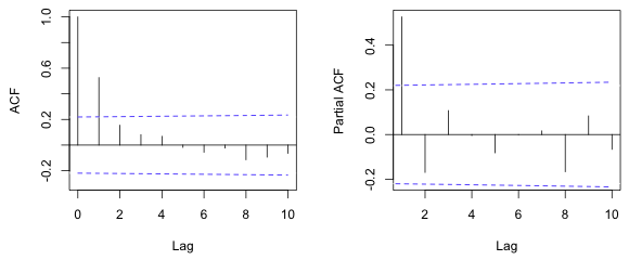
Fig. 5 ACF and PACF of an ARMA(1,1) process (R code)
| Pattern | Conclusion |
| ACF exhibits no significant spikes. Spikes at all lags are near zero. | Uncorrelated |
Uncorrelated processes may exhibit some decay over time, but none of the correlations at any lag will be statistically significant. In order for this to be true it may be necessary to carry out a Bonferroni correction to obtain the appropriate familywise α-level. In carrying out a Bonferroni correction the desired alpha level (typically α = .05) is divided by the number of lags that are being examined. One should only include the lags in this calculation for which the sample size is adequate to accurately estimate a correlation.
| Pattern | Conclusion |
| ACF exhibits significant spikes at roughly regular intervals. | Periodic process |
The potential for periodicity in temporal data can usually be anticipated a priori and should have a theoretical basis. If a periodic process is observed in the residuals of a regression model, a periodic function of time (consisting of both a sine and cosine term) can be included in the regression model.
| Pattern | Conclusion |
| ACF exhibits many significant spikes that fail to decay or that decay only extremely gradually. | Process is not stationary. |
If the temporal correlation of the regression residuals fails to decay over time, it means that the regression model is inadequate. There is a trend over time that has not been accounted for. If no further time-dependent predictors are available for inclusion in the regression model, various functions of time can be added to the model until the residuals exhibit stationarity.
The R code used to generate Figs. 3–5 and the output contained in this document appears here.
| Jack Weiss Phone: (919) 962-5930 E-Mail: jack_weiss@unc.edu Address: Curriculum for the Environment and Ecology, Box 3275, University of North Carolina, Chapel Hill, 27599 Copyright © 2012 Last Revised--February 15, 2012 URL: https://sakai.unc.edu/access/content/group/2842013b-58f5-4453-aa8d-3e01bacbfc3d/public/Ecol562_Spring2012/docs/lectures/lecture16.htm |