Final Exam—Solution

Problem 1

Question 1

We need to fit a Poisson random intercepts model so we can adapt the comparable code from lecture 25. The variable Season is the grouping variable for the random effects. I read in the data and create the objects needed for WinBUGS and JAGS.

The BUGS program is shown below.

Fig. 1   Trace plots of individual Markov chains for each parameter.

Question 2

The percentile and HPD 95% credible intervals are shown below. I've highlighted the intervals that correspond to the coefficient of log(Tows).

When we include log(Tows) as an offset in a model we are fixing its coefficient to be 1 rather than estimating it. To determine if this is a good idea we can carry out a hypothesis test.

H₀: b4 = 1
H₁: b4 ≠ 1

An equivalent way of carrying out this test is to construct a confidence interval for b4. We fail to reject H₀ at α = .05 if 1 is not in a 95% confidence interval for b4. The reported 95% credible intervals are percentile: (0.305, 1.072) and HPD: (0.274, 1.02). Because the number 1 is contained in both the percentile and HPD 95% credible intervals we fail to reject 1 as a possible value for the coefficient of log(Tows) in the model. Therefore treating log(Tows) as an offset with a coefficient of 1 is a reasonable thing to do here.

Problem 2

Question 1

The three design features that are deviations from an ordinary two-factor design with crossed factors are the following.

1. This is a split plot design for the temperature treatment.
2. There are repeated measures for the time effect
3. We need to include a covariate to control for differences in initial size.

Split plot design. Although the growth of individual animals was tracked over time, the main treatment of interest, temperature, was randomly applied to nine different aquaria, not to the 9 × 18 = 162 individual animals in the study. If this had been a true factorial design then each coral would have been placed in an individual jar with its own thermostat. 54 of the jars would have been randomly assigned to the 25°C treatment, 54 jars would have been randomly assigned to the 28°C treatment, and 54 jars would have been randomly assigned to the 32°C treatment. For logistical reasons this wasn't done and treatments were randomly assigned to aquaria. Corals from the same tank would be expected to be more similar to each other than to corals from different tanks, not only because they share a common temperature treatment but because they share a common aquarium environment. As a result the observations used in the study are not all equivalent, something we've called data heterogeneity. In the language of split plot designs the aquarium is the whole plot unit, the individual corals are the split plot units, and temperature is the whole plot treatment. Technically there is no split plot treatment here. Analytically we can account for the split plot design by fitting a mixed effects model. The grouping variable in the mixed effects model is tank.grp, a variable that uniquely identifies each of the nine aquaria. (Note: Technically because there is no split plot treatment we would usually call the temperature experiment a nested design rather than a split plot design but the method of analysis is the same.)

Repeated measures design. There are 486 observations in the data frame coming from 162 different animals with three measurements per animal. Thus we don't have a random sample of animal times. If this had been a random sample of animal-times then there would have been 486 animals of which 162 would have been randomly chosen to be measured at time 1, a different 162 chosen to be measured at time 2, and the remaining 162 chosen to be measured at time 3. Instead we measured each animal three times. Thus we have measurements from the same animal as well as measurements from different animals. We would expect measurements made on the same animal to be more similar to each other than they are to measurements made on different animals. Thus we have observational heterogeneity. The grouping variable here is the individual animal, recorded as the variable id in the data frame. A repeated measures design can be analyzed like a split plot design. The animal (id) is the whole plot unit and the individual time measurements on that animal (the rows of the data frame) are the split plot units. There are no treatments per se unless time is viewed as a treatment.

The temperature experiment combined with the repeated measures together can be viewed as a split-split plot design. In this perspective aquaria are whole plot units, individual corals are split plot units, and the individual time measurements are split-split plot units. Temperature is the whole plot treatment and time can be viewed as a split-split plot "treatment", but that's a bit of a stretch. Once again there is no split plot treatment.

Controlling for a nuisance covariate. Because the animals did not all have the same initial size, it is necessary to include the variable surf.area as a covariate to control for differences in size. In its simplest form this would convert a two-factor analysis of variance model to test for the effects of temperature, time, and their interaction, into an analysis of covariance model that also includes the additive effect of surf.area. It is possible that the effect of treatment also varies with the value of the covariate. This should be investigated by fitting a preliminary model in which surface area is allowed to interact with the treatment variables.

Question 2

The grouping variables are tank.grp, the unique identifier for the nine aquaria, and id, the unique identifier for the individual coral animals. Using the nlme package we would represent this structure with random=~1|tank.grp/id. Using the lme4 package we just need to include the terms (1|tank.grp) + (1|id). Because this is a controlled experiment where all detected effects should be only due to the administered treatments we should start with the most complicated model, one that includes an interaction between temp, time.period, and surf.area. To avoid confusion I convert both temp and time.period to factors before fitting the model.

Using the lme4 package, the model would be written as follows.

Question 3

I use with the nlme package for the analysis because it's easier to use with normal-response mixed effects models.

According to the ANOVA table we can drop the three-factor interaction. I refit the model with all two-factor interactions.

When time.period:surf.area is added last it is not significant so we can drop it.

Changing the order of the two-factor interaction terms in the sequential ANOVA table does not affect our conclusions. All of the remaining effects are statistically significant.

Note: There was actually no need to refit the model. We could have used anova(out.lme3, type='marginal') to obtain marginal tests of each effect.

Question 4

There are three different ways to obtain treatment means, their standard errors, and confidence intervals. We can

1. reparameterize the model to return means directly and then use the intervals function from the nlme package,
2. use the effects package with the original model, or
3. construct a contrast matrix to obtain the means and standard errors.

I illustrate each method in turn.

Method 1: Reparameterize the model and use the intervals function

The first two hints for this question suggest reparameterizing the model so that we can get the means we want directly rather than their effects. The means of interest correspond to the temp:time.period interaction. Following the hint I fit a model with only the two 2-factor interactions and no intercept. I also center surface area at 10 using the I function of R.

The AIC of this model matches the AIC of the model in its original parameterization indicating that they're equivalent.

If we examine the summary table of the model we can see that we've obtained what we want.

When we plug in surface area = 10, the last three terms in the model will drop out. The first nine terms are the means at the individual temperatures and time periods. To get the confidence intervals I use the intervals function on this model with the which="fixed" argument so that we only get confidence intervals for the fixed effect estimates. The entries we want are in the first nine rows.

Method 2: Use the effects package

To use the effects package to obtain the means we can use the original model. The syntax for obtaining the means at each temperature and time combination when surface area = 10 is the following.

The terms we want are scattered in different components of the object returned by the effect function.

Notice that the confidence bounds are slightly different from what we obtained using the first method. That's because the intervals function uses a t-distribution with 316 degrees of freedom (see the summary table above) in calculating the confidence bounds while the effects package uses a normal distribution. We can easily demonstrate this fact.

Method 3: Hand calculation

This method was outlined in lecture 4. To obtain the means at the nine different combinations of temperature and time we form the matrix product Cβ where the nine rows of C contain the values of the regressors in the model at each of those means and β is the vector of fixed effect estimates from the model, fixef(out.lme3). The variance-covariance matrix of the means can be obtained with the matrix product , where Σ_β is the variance covariance matrix of the parameter estimates obtained with vcov(out.lme3). The second appearance of C in the product is the matrix transpose of the first. To obtain the standard errors of the means we extract the diagonal of the final matrix and take its square root.

I start by using expand.grid to obtain the nine combinations of temperature and time that correspond to the nine means.

I next create the dummy variables for temperature and time that correspond to these nine observations. An easy way to get them is with the outer function, which can be used to carry out element-wise calculations on two sets of vectors. Here I test separately whether the temperature is equal to 28 or to 32.

I do a similar calculation for time.

I examine the entries of the coefficient vector from the model.

We need to construct a matrix C with 12 columns so that each column corresponds to a different regressor. I start by adding the intercept, the dummy vectors for temperature, the dummy vectors for time, and a column for surface area = 10.

Next I create the interactions by multiplying the corresponding dummy vectors together. I do this so that the results match the order shown in the coefficient vector.

Next I use the matrix C to calculate the means and their standard errors. I then obtain the lower and upper 95% confidence intervals for the means using a t-distribution for the multiplier just like the intervals function does.

The matrix of results matches what we obtained using the intervals function in Method 1. 

Question 5

Because this is a repeated measures design I place time on the x-axis and draw separate time profiles for each temperature. There are two sensible graphs we could produce here. We can put the time profiles for each temperature in a single panel or in different panels. I illustrate both approaches.

Method 1: One-panel graph

I modify the code from Lecture 8 that uses a group panel function. In lecture 8 there were only two groups. Here we have three. I start by collecting the factor levels and estimates in a data frame.

Because the graph is rather full, I don't do a legend but instead use the panel.text function to place an identifier for each temperature at the end of its corresponding profile. To get the correct temperature to show up on the correct profile with a degree symbol, I use the substitute function, something that we didn't cover in the course. The substitute function allows one to insert the values of variables into mathematical expressions.

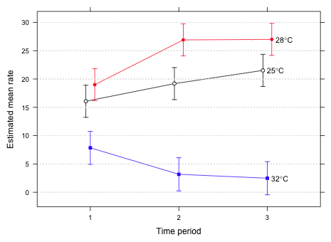Fig. 2   Interaction graph in a single panel

Method 2: Three-panel graph

For this method I place each time profile in a separate panel according to its temperature.

To get degree symbols in the panel strips takes a bit of work. If we're sure of which label goes where we can hardwire it in with the strip.custom function in the strip argument. I use the factor.levels argument to specify formatted values for the temperature in a specific order.

A more elegant approach is to do this dynamically and let the xyplot function figure out what temperature labels go where. For this we have to write a function that substitutes a value of temperature into a math expression. Then we have to use the strip argument with the strip.custom function to apply this function to the value for each panel separately.

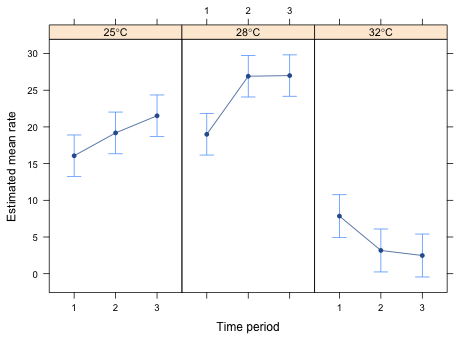Fig. 3   Interaction graph in three panels

Problem 3

Question 1

Define a dummy variable for Morph.

The regression model that answers the researcher's question is a model that includes distance, a dummy variable for Morph, and the interaction between the two of them.

Question 2

The goal is to find evidence of natural selection on moth color morphs based on the background color of tree bark. Distance from Liverpool is the proxy for tree background color. The greater the distance the lighter the bark. If we can show that the distance from Liverpool affects the removal rate of the two color morphs differently that would be evidence that the combination of moth color and bark color matters.

We have two regression models depending on the Morph. When Morph = 'dark', (z = 0), we have

When Morph = 'light', (z = 1), we have

On the scale of the response these expressions represent two lines with different slopes and different intercepts. The relationship with distance is the same if the two slopes are the same. This would happen if β₃ = 0. Thus our null hypothesis stated in terms of the regression model is simply H₀: β₃ = 0.

Question 3

The response variable is the number of moths removed out of a fixed total. A suitable probability model is a binomial distribution and hence logistic regression is appropriate.

Deviance Residuals:
     Min        1Q    Median        3Q       Max 
-2.21183  -0.39883   0.01155   0.68292   1.31242 

Coefficients:
                     Estimate Std. Error z value Pr(>|z|)   
(Intercept)         -1.128987   0.197906  -5.705 1.17e-08 ***
Morphlight           0.411257   0.274490   1.498 0.134066   
Distance             0.018502   0.005645   3.277 0.001048 **
Morphlight:Distance -0.027789   0.008085  -3.437 0.000588 ***
---
Signif. codes:  0 ‘***’ 0.001 ‘**’ 0.01 ‘*’ 0.05 ‘.’ 0.1 ‘ ’ 1

(Dispersion parameter for binomial family taken to be 1)

    Null deviance: 35.385  on 13  degrees of freedom
Residual deviance: 13.230  on 10  degrees of freedom
AIC: 83.904

Number of Fisher Scoring iterations: 4

The interaction is significant so we have evidence that the predation rate varies with distance in a different manner for the two morphs. From the output the predation rate for the dark morph increases with distance. The significant interaction tells us that the change in the predation rate with distance for the light morph is significantly less than it is for the dark morph. To understand this better we can force R to return separate slopes for each Morph type by refitting the model without the main effect of Distance.

Now we see that for the dark morph the predation rate increases with distance (slope = 0.0185) and the relationship is significant (p = 0.001). For the light morph the predation rate decreases with distance (slope = –0.0093), although the relationship is not statistically significant (p = 0.109). The signs of the coefficients are consistent with theory. The further away from Liverpool we are the lighter the trees are thus making the dark morph more vulnerable to predation and the light morph less so.

Question 4

The residual deviance can be used as a goodness of fit statistic if the predicted counts are large enough, greater than 5. Checking this we find that all the predicted counts are greater than 5.

I compare the residual deviance to a chi-squared distribution with degrees of freedom equal to the residual degrees of freedom.

The residual deviance is not significant. Therefore we fail to find evidence of lack of fit.

Question 5

The experiment is set up in the form of a randomized block design. At each of the seven location we have pairs of observations: the light morph binomial result and the dark morph binomial result for a total of 14 measurements. Contrast this with an ordinary crossed design in which case there would be 14 locations and 14 measurements. The fact that we have measurements from the same location and measurements from different locations means that the data are heterogeneous. We should account for the pairing of observations in the analysis.

Question 6

I fit a logistic regression random intercepts model treating Location as the grouping variable. Because Distance varies across Location (but is constant within a Location), Distance is a level-2 predictor. Because Morph varies within a Location, Morph is a level-1 predictor.

Fixed effects:
                     Estimate Std. Error z value Pr(>|z|)   
(Intercept)         -1.130918   0.212723  -5.316 1.06e-07 ***
Morphlight           0.411129   0.274625   1.497 0.134379   
Distance             0.018477   0.006150   3.005 0.002659 **
Morphlight:Distance -0.027819   0.008089  -3.439 0.000584 ***
---
Signif. codes:  0 ‘***’ 0.001 ‘**’ 0.01 ‘*’ 0.05 ‘.’ 0.1 ‘ ’ 1

Correlation of Fixed Effects:
            (Intr) Mrphlg Distnc
Morphlight  -0.672             
Distance    -0.871  0.581      
Mrphlght:Ds  0.570 -0.859 -0.643

Other than a slight increase in the standard errors of the parameter estimates, the results from the mixed effects model are virtually identical to the results from the ordinary logistic regression model.

Question 7

Analysis of deviance

Ordinarily to carry out an analysis of deviance we would subtract the deviance of the two models and compare the result to a chi-squared distribution with 1 degree of freedom (the number of parameters that the two models differ by). The parameter in question is the variance of the random effects, τ², which is set to zero in the ordinary logistic regression model. Because 0 is a boundary value for the variance, the usual distribution for the test statistic is incorrect. What we saw previously in lecture 18 was that the correct distribution can be approximated by a distribution that is approximately a 50:50 mixture of two chi-squared distributions, one with 0 degrees of freedom and one with 1 degree of freedom. Thus we should use a mixture of a and a random variable, each assigned a weight of 0.5.

This translates into dividing the usual p-value of our test by 2.

The test statistic is not significant so we conclude that the two models are not significantly different. Thus there doesn't appear to be a need for the random effects.

Using AIC

Alternatively we can calculate the AIC of the models. The values returned by AIC and logLik for an lmer model cannot be compared to those same values from an ordinary logistic regression model. Following the hint for this question I calculate the log-likelihood of a saturated model. The saturated model has one parameter per observation. I create a factor variable with 14 levels and fit the logistic regression model to it.

Alternatively the formula for the deviance tells us the following.

Solving for the log-likelihood of the saturated model we obtain the following.

Using this formula with the glm model we obtain the following.

which is the same answer we obtained above. Using the deviance expression again I this time solve for the log-likelihood of the model of interest.

For the mixed effects model we estimated four regression parameters plus the variance of the random effects for a total of 5 parameters. Using this and the correct log-likelihood for the lmer model we obtain the following value of AIC.

The AIC of the random effects model is larger than the AIC of the glm model. Once again we find little support for the random effects.

Question 8

Consider two moths both of the dark morph that are 50 km apart. The predicted logits for the two moths are the following.

Subtracting the two expressions yields the following.

If we turn to the light morphs we get the same kind of expression except for light morphs the effect of distance is given by β₂ + β₃.

Subtracting the two expressions and exponentiating the result yields the following.

Plugging in the data we obtain the odds ratios.

So for the dark morph the odds of being removed in North Wales is 2.5 times its odds of being removed in Liverpool. For the light morph the odds of it being removed in North Wales is only 62% of its odds of being removed in Liverpool.

Question 9

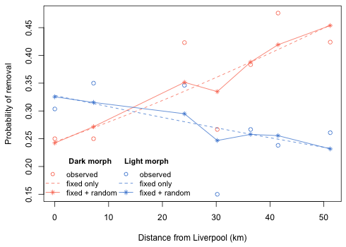Fig. 4   Effect of distance on the probability of removal of individual morphs

The curves labeled "fixed only" correspond to the estimated regression model from the mixed effects model that includes only the fixed effects terms. The trajectories labeled "fixed + random" are the location-specific probabilities obtained by adding the random effects to the already displayed fixed effects curves.

Question 10

The four basic assumptions of the binomial distribution are:

1. The experiment must consist of a sequence of trials in which each trial is a Bernoulli trial, meaning only one of two outcomes with probabilities p and 1 – p can occur.
2. The number of trials is fixed ahead of time at n, a value that is known to us.
3. The probability p is the same on each Bernoulli trial.
4. The Bernoulli trials are independent.

Clearly the first two assumptions still hold. Independence is always an issue with binomial trials, but we need to assume that the researche did not choose to blatantly violate this assumption. If you look at the paper you'll see that the protocol was to put one moth out for a fixed length of time. They then recorded whether during that time it was removed or not. If it was not removed they removed it and put a fresh moth out. This was then repeated until the moth supply was exhausted.

If birds developed a search image over time then perhaps independence might have been an issue in the original design. With multiple trees the same protocol was followed. If anything the use of multiple trees rather than a single tree might actually make it more likely the individual Bernoulli trials were independent.

What the introduction of multiple trees does do is introduce observational heterogeneity. Given that different trees are not likely to be identical in their bark color and other characteristics, the probability of a moth being detected and eaten probably varied from tree to tree. We've been assuming that except for the effect of morph type the probability of being removed was the same for each moth at a location. This might not be the case for different moths if they were on different trees.

Question 11

A simple rule is that the normal approximation to the binomial distribution is likely to hold if both np > 5 and n(1 – p) > 5. I check this for our data. np and n(1 – p) are just the number of moths removed and the number of moths that are left behind.

So both of these values are greater than 5 for every observation. The normal approximation should be reasonable. I analyze the proportions using a randomized block design treating block (location) as a random effect.

Random effects:
 Formula: ~1 | Location
        (Intercept)  Residual
StdDev:  0.05410956 0.0378578

Fixed effects: p ~ Morph * Distance
                          Value  Std.Error DF   t-value p-value
(Intercept)          0.24394502 0.04712545  5  5.176503  0.0035
Morphlight           0.08102398 0.03820586  5  2.120721  0.0874
Distance             0.00401661 0.00146803  5  2.736044  0.0410
Morphlight:Distance -0.00590237 0.00119017  5 -4.959245  0.0043
 Correlation:
                    (Intr) Mrphlg Distnc
Morphlight          -0.405             
Distance            -0.848  0.344      
Morphlight:Distance  0.344 -0.848 -0.405

Standardized Within-Group Residuals:
        Min          Q1         Med          Q3         Max
-0.83172423 -0.66326402 -0.01896693  0.52633610  1.12747315

Number of Observations: 14
Number of Groups: 7

Our conclusions are the same. The probability of being removed increases with distance for the dark morph. This change with distance is significantly less for the light morph where it actually decreases with distance (although not significantly different from zero).

Question 12

I obtain the pairwise differences in the proportion of moths removed for each pair of morphs, dark minus light, at each location and regress them against the location's distance from Liverpool.

Residuals:
  Clergy Mawr Eastham Ferry      Hawarden      Llanbedr   Loggerheads
      0.05813       0.06147      -0.01570       0.01716      -0.01944
    Pwyllglas   Sefton Park
     -0.07417      -0.02745

Coefficients:
             Estimate Std. Error t value Pr(>|t|)  
(Intercept)  0.081024   0.038206   2.121  0.08743 .
out.dist    -0.005902   0.001190  -4.959  0.00425 **
---
Signif. codes:  0 ‘***’ 0.001 ‘**’ 0.01 ‘*’ 0.05 ‘.’ 0.1 ‘ ’ 1

Residual standard error: 0.05354 on 5 degrees of freedom
Multiple R-squared: 0.831,  Adjusted R-squared: 0.7973
F-statistic: 24.59 on 1 and 5 DF,  p-value: 0.004251

Observe that the two rows of the summary table from this model match the two rows in the summary table of the randomized blocks design of Question 11 labeled Morph and Morph:Distance. There Morph represents the difference in removal rate between dark and light Morphs at distance 0 (Liverpool). The interaction in that model represents how much the probability change with distance differs between the two morphs. Both of these are difference estimates. It is always the case that when you analyze paired data as a randomized block design or as a regression on differences (thus removing the block effects) you get identical results for the differences. Of course with the paired difference analysis you can't predict the actual counts at each site, only the difference between them.

The point of Questions 11 and 12 is to note that it is not always necessary to carry out a complicated analysis of data. The old-fashioned methods that were popular before the advent of sophisticated statistical software often work just as well and can be easier for the lay reader to understand.

Course Home Page