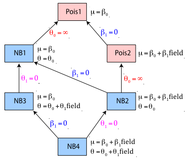
Fig. 1 A hierarchy of Poisson and negative binomial models
I reload the slugs data set from lecture 17 and refit both the common means and separate means Poisson regression models as well as the common means and separate means negative binomial regression models.
There are six models we might consider for the slugs data set: two Poisson and four negative binomial models. Table 1 lists these models.
| Table 1 Regression models for the slugs data set |
Model |
Distribution |
Mean model |
Dispersion model |
Pois1 |
Poisson |
μ = β0 |
— |
Pois2 |
Poisson |
μ = β0 + β1*field |
— |
NB1 |
negative binomial |
μ = β0 |
θ = θ0 |
NB2 |
negative binomial |
μ = β0+ β1*field |
θ = θ0 |
NB3 |
negative binomial |
μ = β0 |
θ = θ0+ θ1*field |
NB4 |
negative binomial |
μ = β0+ β1*field |
θ = θ0+ θ1*field |
So far we've fit four of these. The two models we have yet to consider are NB3 and NB4 that allow the dispersion parameter θ of the negative binomial distribution to vary by field type. We saw in lecture 16 that when the mean of the negative binomial distribution is held fixed smaller values of θ yielded more heterogeneous data, data that can exhibit a large number of zero counts along with some extremely large counts. From an ecological perspective, low values of θ correspond to environmental patchiness such that many locations yield no individuals but some locations are teeming with individuals.
With only one predictor at out disposal, field type, Table 1 exhausts the possibilities when we restrict ourselves to Poisson and negative binomial distributions. Because the likelihood for each model is the probability of obtaining the data if that particular model is the correct model, we can carry out an informal comparison of the Poisson and negative binomial models by comparing their log-likelihoods.
The log-likelihoods aren't directly comparable because some of the models use different numbers of parameters. But if we examine the two 2-parameter models, the separate means Poisson model, out.pois2, and the common mean negative binomial model, out.NB1, we see that the log-likelihood of the negative binomial model (–144.398) is much greater than the log-likelihood of the Poisson model (–171.1275). This suggests that the negative binomial distribution is a more likely model for these data.
Because a number of the models shown in Table 1 are nested we can formally compare them with a likelihood ratio test. Given a pair of nested models the likelihood ratio test can be used to determine whether the more complicated model can be reduced to the simpler model. A significant result for the likelihood ratio test indicates that the simplification should not be carried out meaning we should prefer the more complicated model over the simpler model. Fig. 1 below shows the hierarchical relationships between the six models of Table 1.
Fig. 1 A hierarchy of Poisson and negative binomial models
Fig. 1 is a directed graph that shows the pathways along which likelihood ratio tests can be used to compare pairs of models. Any two models that can be reached by following the arrows in the direction shown in Fig. 1 can also be legitimately compared using a likelihood ratio test. The arrows in the figure point in the direction of model simplification. The hypothesis tested by the likelihood ratio test is indicated next to the arrow that connects the models. So, for instance, model Pois2 can be reduced to Pois1 if the coefficient of field type, β1, in the regression model for the mean is not significantly different from zero. The likelihood ratio test is carried out by comparing the log-likelihoods of the two models.
Fig. 1 also indicates possible comparisons among the four negative binomial models. We can compare NB4 with NB2, NB2 with NB1 (and therefore NB4 with NB1), NB4 with NB3, and NB3 with NB1. Notice that it is not possible to compare models NB3 and NB2 because there is no pathway connecting them in the direction of the arrows. This follows from the fact that the models are not nested. Model NB2 contains the parameter β1 not found in NB3 while model NB3 contains the parameter θ1 not found in NB2. We have to hope instead for an indirect test, one in which a likelihood ratio test we can carry out allows us to reject one of these models in favor of a competing model. If it turns out that the available likelihood ratio tests do not reject either NB3 or NB2 then there is no way to discriminate between them using significance testing. In lecture 19 we will discuss an alternative to significance testing that does allow us to compare models NB3 and NB2 directly.
There are two other tests possible in Fig. 1, the tests that compare NB2 with Pois2 and NB1 with Pois1 and allow us to choose between a negative binomial and a Poisson model. These tests turn out not to be straight-forward likelihood ratio tests. The details are discussed in the next section.
The negative binomial and Poisson distributions differ in a single parameter, the dispersion parameter θ. In lecture 15 it was mentioned that the Poisson distribution can be thought of as a limiting case of the negative binomial distribution. As θ → ∞, the negative binomial distribution approaches a Poisson distribution with the same mean. The other common way to parameterize the negative binomial is with a parameter![]() . With this parameterization we don't have to invoke limits. The Poisson distribution corresponds to a negative binomial distribution in which α = 0. Consequently using this parameterization a Poisson model and a negative binomial model with the same mean are clearly nested.
. With this parameterization we don't have to invoke limits. The Poisson distribution corresponds to a negative binomial distribution in which α = 0. Consequently using this parameterization a Poisson model and a negative binomial model with the same mean are clearly nested.
A formal test of whether the negative binomial distribution is an improvement over the Poisson distribution might take the following form.
The alternative hypothesis is one-sided because the dispersion parameter can't be negative. To carry out the test of this hypothesis we could construct a likelihood ratio statistic, twice the difference in the log-likelihoods of the two models.
![]()
Because the two models are nested and differ in the presence of a single parameter, θ, we would ordinarily compare the value of LR to the critical value of a chi-squared distribution with one degree of freedom. If it turns out that ![]() (or alternatively that the p-value of our test statistic is small), we would reject the null hypothesis and conclude that the negative binomial model is preferred over a Poisson model.
(or alternatively that the p-value of our test statistic is small), we would reject the null hypothesis and conclude that the negative binomial model is preferred over a Poisson model.
Unfortunately the likelihood ratio test just described is incorrect. The null hypothesis being tested asserts that the dispersion parameter α is zero. Because dispersions can't be negative, a value of zero is a boundary value of the parameter space of α. One of the conditions for the asymptotic chi-squared distribution of the likelihood ratio statistic to hold is that the value being tested does not lie on the boundary of the parameter space. This is referred to as a regularity condition. Because the regularity condition fails in a test that compares a negative binomial distribution with a Poisson distribution the chi-squared distribution ( ![]() ) of the likelihood ratio statistic is suspect.
) of the likelihood ratio statistic is suspect.
A number of solutions to this situation have been proposed. One that is easy to implement is from Verbeke and Molenberghs (2000), p. 64–7, who discuss it in the context of mixed effects models, a topic we'll discuss later in the course. They argue that the distribution of the likelihood ratio statistic for testing a boundary condition can be approximated by a mixture distribution that is approximately a 50:50 mixture of two chi-squared distributions, one with 0 degrees of freedom and one with 1 degree of freedom. Thus we should use a mixture of a ![]() and a
and a ![]() random variable, each assigned a weight of 0.5, as the critical value of our test.
random variable, each assigned a weight of 0.5, as the critical value of our test.
![]()
A ![]() random variable gives a probability mass of 1 to the value 0 and a mass of 0 to every other value. It's what's called a point mass function. The cdf of a
random variable gives a probability mass of 1 to the value 0 and a mass of 0 to every other value. It's what's called a point mass function. The cdf of a ![]() random variable is 0 for x < 0 and 1 for every value of x > 0. In Fig. 2 the notation 0– means a value just a little bit less than 0, while the notation 0+ denotes a value just a little bit bigger than 0.
random variable is 0 for x < 0 and 1 for every value of x > 0. In Fig. 2 the notation 0– means a value just a little bit less than 0, while the notation 0+ denotes a value just a little bit bigger than 0.
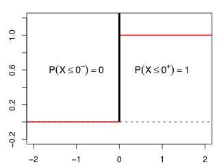
Fig. 2 The pdf (black) and cdf (red ) of a ![]() distribution
distribution
Using this mixture distribution the critical value of our test statistic is
If we calculate the likelihood ratio test statistics for a comparison of NB2 with Pois2 and NB1 with Pois1, we find that the observed values of both test statistics exceed this critical value.
Thus we reject the null hypothesis and conclude that a negative binomial model is a significant improvement over a Poisson model in both cases. As Fig. 2 shows if LR > 0 then P(![]() ≤ LR) = 1 and hence P(
≤ LR) = 1 and hence P(![]() > LR) = 0. So the contribution of this term to the p-value of our test statistic is zero. The p-values of the two tests can be calculated as follows.
> LR) = 0. So the contribution of this term to the p-value of our test statistic is zero. The p-values of the two tests can be calculated as follows.
The p-values are exceedingly small causing us to reject the null hypothesis that α = 0.
Although we found that the mean slug counts in the two fields were significantly different under a separate means Poisson model (using a likelihood ratio test that compared Pois1 with Pois2), the analytical goodness of ft test we carried out in lecture 17 showed that the separate means Poisson model does not fit the data. We saw in the previous section that the negative binomial models NB1 and NB2 are a significant improvement over the Poisson models, but we also saw in lecture 17 that when we use an LR test to compare models NB1 and NB2 we found that they were not significantly different indicating that if slug counts have a negative binomial distribution then the mean slug occurrence is not significantly different across field types. This still leaves open the possibility that the dispersion parameter of the negative binomial distribution varies by field type.
In a Poisson model there is only a single parameter, the rate, so our only choice was to use field type to model the rate. The negative binomial model has two parameters and we can choose to let one or both of them to differ by field type. So far we've just built a model for the mean. Another possibility is to model the dispersion parameter. In the code below the dispersion parameter, theta, is allowed to vary by field type but the mean is kept constant.
$estimate
[1] 2.0913794 0.2506018 1.6472297
$gradient
[1] 1.479944e-05 6.480150e-05 -6.729157e-06
$code
[1] 1
$iterations
[1] 16
The common mean and dispersion negative binomial model, out.NB1, fit previously is nested in out.NB3, so we can test whether the dispersion parameter is the same in both field types using a likelihood ratio test.
Model NB1 |
Model NB3 |
 |
 |
The likelihood ratio test is a test of the following.
H0: θ1 = 0
H1: θ1 ≠ 0
So we reject the null hypothesis and conclude that the dispersion parameters are significantly different between the two habitats. One way to interpret a difference in the dispersion parameter is that in the habitat with the lower dispersion parameter (Nursery) the slugs are more clustered than in the other habitat (Rookery). In the nursery habitat most of the rocks examined had no slugs under them so the distribution of slugs was patchier.
The last model we consider is a negative binomial model in which both the mean and the dispersion are allowed to vary by field type. The code to fit this model is shown below.
$estimate
[1] 1.2750057 0.9999968 0.2840913 1.6448438
$gradient
[1] 6.210394e-05 2.464162e-05 1.243734e-04 -1.128337e-05
$code
[1] 1
$iterations
[1] 21
Models NB3 and NB4 are directly comparable using a likelihood ratio test because model NB3 is contained in NB4. Model NB4 has an additional parameter β1.
Model NB3 |
Model NB4 |
|
 |
The likelihood ratio test here is a test of the following.
H0: β1 = 0
H1: β1 ≠ 0
We fail to reject the null hypothesis and conclude that the means are not significantly different between the two habitats. Thus we should retain the simpler model NB3 and reject model NB4. For future reference I collect the log-likelihoods and the number of estimated parameters for all six of the models that we've fit.
We've already seen that Poisson models can be fit with the glm function and negative binomial models for the mean can be fit with the glm.nb function from the MASS package. To fit negative binomial models in which the dispersion parameter is modeled we can use the gamlss function from the gamlss package. I briefly review fitting the glm and glm.nb models but then focus on fitting the gamlss models.
The glm function fits Poisson models with a log link so that it models log μ. We can override that and force glm to fit models to μ by explicitly specifying an identity link.
Generally speaking there is no reason to use an identity link and every reason not to. The use of the log link guarantees that the regression model will yield a positive value for μ, something that is necessary because μ is the mean of counts. One consequence of using a log link is that the coefficients have a different interpretation. Consider the separate means Poisson model with a log link.
So although the predictors act additively on the scale of log mean, they have a multiplicative effect on the scale of the raw mean. Thus the effect on the mean of switching from nursery to rookery is to multiply the mean by exp(β1) = 1.78.
The MASS package can be used to fit negative binomial models for the mean. As with Poisson regression the default link function is a log link. Consequently regression coefficients for the default negative binomial model have a multiplicative interpretation.
The gamlss package is a comprehensive package for fitting regression models using a vast array of probability models. The gamlss package allows the user to model any of the parameters of these distributions, not just the mean. The name gamlss is short for "generalized additive models for location, scale, and shape." The gamlss package has its own web site with extensive documentation (www.gamlss.org).
If you examine the help screen for gamlss and then click the link for the help screen of gamlss.family, you'll see the basic syntax for gamlss and the probability models it supports. The negative binomial distribution we've been fitting is denoted NBI by gamlss and is specified in a family argument. (There is a second negative binomial distribution that is denoted by NBII that we may have a chance to talk about at a later date.) The gamlss function has separate arguments for specifying the regression model for each parameter. The mean argument is denoted mu.formula and is the first argument of the function while the regression model for the dispersion parameter is specified in the sigma.formula argument.
NB3: Common mean, separate dispersions modelTo fit the common mean, separate dispersions model with gamlss we would write the following.
This fits the following models for the negative binomial parameters
gamlss model NB3 |
 |
The gamlss function uses a log link for both the mean and the dispersion. In addition, gamlss follows the convention of many packages of modeling the reciprocal of the glm.nb θ parameter, ![]() . As a result α = 0 corresponds to a Poisson distribution and larger values of α indicate overdispersion. To see the detailed output from the analysis we use the summary function on the fitted model.
. As a result α = 0 corresponds to a Poisson distribution and larger values of α indicate overdispersion. To see the detailed output from the analysis we use the summary function on the fitted model.
slugs
*******************************************************************
Family: c("NBI", "Negative Binomial type I")
Call: gamlss(formula = slugs ~ 1, sigma.formula = ~field, family = NBI,
data = slugs)
Fitting method: RS()
-------------------------------------------------------------------
Mu link function: log
Mu Coefficients:
Estimate Std. Error t value Pr(>|t|)
(Intercept) 0.7378 0.1432 5.152 1.855e-06
-------------------------------------------------------------------
Sigma link function: log
Sigma Coefficients:
Estimate Std. Error t value Pr(>|t|)
(Intercept) 1.384 0.3602 3.842 0.0002469
fieldRookery -2.024 0.6083 -3.328 0.0013362
-------------------------------------------------------------------
No. of observations in the fit: 80
Degrees of Freedom for the fit: 3
Residual Deg. of Freedom: 77
at cycle: 4
Global Deviance: 276.4796
AIC: 282.4796
SBC: 289.6256
*******************************************************************
Warning message:
In summary.gamlss(glm.NB3) :
summary: vcov has failed, option qr is used instead
The estimates for the mean model and the dispersion model appear in separate sections of the output. The warning message at the bottom means that gamlss was unable to extract the variance-covariance matrix of the parameter estimates, so it used an approximate method, denoted qr, to obtain the standard errors. This seems to happen a lot with this function. According to the documentation when this happens the reported standard errors should be used with caution. Using the coef function on a gamlss model returns the parameter estimates from the mean formula.
The gamlss package includes a special method for coef that permits the inclusion of a what argument to extract the estimates for the dispersion part of the model.
We can map these results onto those returned by nlm as follows.
To match the overall mean returned by nlm we need to exponentiate the value returned by gamlss.
To obtain the dispersion of the "Nursery" habitat we exponentiate the first estimate returned by gamlss and then take the reciprocal of the result.
The dispersion in the "Rookery" habitat is the sum of the two parameters returned by nlm.
To obtain the same value using gamlss we sum the two values it returns, exponentiate the result, and then take the reciprocal.
NB4: Separate means, separate dispersions model
To fit the separate means and dispersions model with gamlss we would write the following.
This fits the following models for the negative binomial parameters.
gamlss model NB4 |
 |
slugs
*******************************************************************
Family: c("NBI", "Negative Binomial type I")
Call: gamlss(formula = slugs ~ field, sigma.formula = ~field, family = NBI,
data = slugs)
Fitting method: RS()
-------------------------------------------------------------------
Mu link function: log
Mu Coefficients:
Estimate Std. Error t value Pr(>|t|)
(Intercept) 0.2429 0.3282 0.7403 0.4613
fieldRookery 0.5790 0.3628 1.5959 0.1146
-------------------------------------------------------------------
Sigma link function: log
Sigma Coefficients:
Estimate Std. Error t value Pr(>|t|)
(Intercept) 1.258 0.4374 2.876 0.005184
fieldRookery -1.915 0.6569 -2.916 0.004631
-------------------------------------------------------------------
No. of observations in the fit: 80
Degrees of Freedom for the fit: 4
Residual Deg. of Freedom: 76
at cycle: 2
Global Deviance: 274.2505
AIC: 282.2505
SBC: 291.7787
*******************************************************************
Warning message:
In summary.gamlss(glm.NB4) :
summary: vcov has failed, option qr is used instead
If we can trust the standard errors and tests that are reported it appears that the dispersion parameter varies across habitat type, but the mean does not.
Finally I collect the results of the various model fits in a single data frame. The log-likelihoods can be extracted with the logLik function. To get all six log-likelihoods simultaneously I create a list object of the models and then sapply the logLik function on the list.
Obtaining the number of parameters k is a bit more awkward because some of the parameters are stored in different components of the model.
So, the results obtained with nlm match the results obtained with glm, glm.nb, and gamlss.
I repeat Fig. 1 below, the directed graph that shows the pathways along which likelihood ratio tests can be used to compare the various models we've fit.
Fig. 1 (again) A hierarchy of Poisson and negative binomial models
The slugs data set is really an observational data set, not an experiment. We don't have treatments per se that were randomly assigned to observational units unless we can view habitat assignment as a random act of nature. Before collecting the data we don't know much about the nature of the response variable except that it is a count. In particular we don't know whether one probability distribution will make more sense here than another. With experimental data in which treatments are randomly assigned to subjects and we can therefore infer causation from correlation, my preference is to start with the most complicated model involving all the treatments and then see if it can be simplified. My rationale is that any treatment effects uncovered from experimental data have a high probability of being real. With observational data the danger of finding spurious relationships by chance is very high. Here, my predilection is to start with the simplest possible model and make it more complicated only if necessary.
So, for the slugs data set I would start with the model labeled Pois1 at the top of the diagram in Fig. 1. According to the diagram there are two ways we can proceed from Pois1. We can try complexifying it by letting the Poisson mean vary by field type (Pois2) or we can add a dispersion parameter and thus replace the Poisson distribution with a negative binomial distribution (NB1).
I start by comparing models Pois1 and Pois2. Because Pois2 is the more complicated model and contains model Pois1, a likelihood ratio test is appropriate. The LR test here tests whether the additional parameter in Pois2 is different from zero.
H0: β1 = 0
H1: β1 ≠ 0
We can carry out this test with the anova function applied to the two glm models.
Model 1: slugs ~ 1
Model 2: slugs ~ field
Resid. Df Resid. Dev Df Deviance Pr(>Chi)
1 79 224.86
2 78 213.44 1 11.422 0.000726 ***
---
Signif. codes: 0 ‘***’ 0.001 ‘**’ 0.01 ‘*’ 0.05 ‘.’ 0.1 ‘ ’ 1
Because the simpler model and the more complicated model are significantly different we conclude β1 ≠ 0 and thus we have reason to prefer the more complicated model, Pois2. Alternatively we can carry out the LR test ourselves, by doubling the difference in the log-likelihoods and using as degrees of freedom the difference in the number of estimated parameters in the two models. We can extract the number of estimated parameters directly from the output of the logLik function. The object created by logLik has an attribute called 'df', for degrees of freedom, that can be extracted with the attr function.
I collect this all in a function that mimics anova and returns the p-value of the test.
This is a non-standard likelihood ratio test because it involves testing whether the dispersion parameter, θ, is equal to a boundary value, ∞.
H0: θ0 = ∞
H1: θ0 < ∞
As was discussed above the p-value for this test is calculated as ![]() .
.
The p-value tells us that the models are significantly different indicating that θ0 < ∞. So, we should choose the more complicated model, NB2, a negative binomial with separate means that vary by field type.
The likelihood ratio test here tests whether the dispersions in the two field types are different given that the means are different.
H0: θ1 = 0
H1: θ1 ≠ 0
We can't use the anova function to compare these models because one model was fit using glm.nb (NB2) and the other using gamlss (NB4). (Also the gamlss package does not have a method for the anova function.) On the other hand the logLik function works with both models so we can carry out the calculation by hand or use the function we previously wrote for this purpose.
So the models are significantly different indicating θ1 ≠ 0. So, we should choose the more complicated model, NB4, a negative binomial model with separate means and separate dispersions depending on field type.
The likelihood ratio test here tests whether the means vary by field type given that their dispersions are different.
H0: β1 = 0
H1: β1 ≠ 0
Both of these models were fit using gamlss. The gamlss package does not have a method for anova but it does have its own function LR.test for carrying out likelihood ratio tests.
Alternatively we can carry out the test ourselves.
So the models are not significantly different and we fail to reject the hypothesis that β1 = 0. Thus we have no reason to prefer the more complicated model (NB4) over the simpler model (NB3). Thus we should choose NB3.
We can ask whether the model with a single mean can be reduced further by letting it have a single dispersion parameter.
H0: θ1 = 0
H1: θ1 ≠ 0
This reduction is unlikely given our previous results from testing NB2 versus NB4. Because we have to compare a gamlss model with a glm.nb function we need to do the calculations by hand.
The models are significantly different and we conclude that θ1 ≠ 0: the coefficient of the field term in the dispersion model is different from zero. Thus we should retain the more complicated model (NB3) over the simpler model NB1. This brings us to a stopping point on pathway 1. NB3 is our final model because we cannot simplify it (the results of the current test) and according to the previous test there is no need to complexify it further by letting the means vary by habitat type.
When we reached model NB2 in the previous pathway we had a choice. We could test NB2 against NB4 (which was the choice we made) or NB2 against NB1. The latter is a test of the separate means model versus the common means model when both models are negative binomial. The corresponding hypothesis test is the following.
H0: β1 = 0
H1: β1 ≠ 0
Because NB1 and NB2 are both glm.nb models the test can be computed with the anova function.
Response: slugs
Model theta Resid. df 2 x log-lik. Test df LR stat. Pr(Chi)
1 1 0.7155672 79 -288.7961
2 field 0.7859313 78 -285.3500 1 vs 2 1 3.446124 0.06340028
The models are not significantly different therefore we fail to reject H0: β1 = 0. Thus we should prefer the simpler model NB1. In Step 5 of Pathway 1 we then discovered that NB3 was a significant improvement over NB1 so we would next choose model NB3 at which point we reach the same stopping point as before.
Initially we had a choice of comparing Pois1 against Pois2 or Pois1 against NB1. If we choose to test Pois1 against NB1 we are testing
H0: θ0 = ∞
H1: θ0 < ∞
This is a non-standard likelihood ratio test because we're testing a boundary value of the parameter space of θ. As was discussed above the p-value of the likelihood ratio statistic for this test is ![]() .
.
The models are significantly different and we conclude θ0 < ∞. So, we should choose the more complicated model, NB1, a negative binomial with a common mean, over the Poisson model with a common mean. At this point in Pathway 1, we next rejected NB1 in favor of NB3 at which point we reached our final model NB3.
So regardless of the pathway we follow we end up with the same model NB3 as our final model, a negative binomial model with a single mean and separate dispersion parameters for the two field types. To assess the fit of this model visually I obtain the probability estimates of the various count categories using this model and superimpose the model predictions on a bar plot of the raw data. The protocol for doing so follows almost exactly what we did for the Poisson model in lecture 16. I start by extracting the mean and dispersions for each field type and adding them to the slugtable data frame. I choose to use the output from nlm, out.NB3, because it doesn't require back-transforming things.
Using these means and dispersions I calculate the negative binomial probabilities of the count categories 0 through 10 for each field type.
The probabilities don't sum to one. I add the tail probability to the last observed count category, X = 10, and store the final probabilities in the column labeled p2.
I next obtain the total sample sizes in each field type.
For these data the sample sizes are the same in the two groups. For other data sets they will be different. One way we can automatically add the sample totals to the slugtable data frame so that the correct total is added to the correct field type is to perform a many-to-one merge. I relabel the variables in the sample size data set, n.data, so that the field variable has the same name in both n.data and slugtable: Var2.
To combine the two data frames I use the merge function of R. The merge function adds the variables of one data frame to a second data frame using the values of a key field that appears in both data frames to link up the correct observations. For us Var2 will serve the role of the key field. The values of the key field have to be all different in at least one of the data frames. This is the case for n.data.
Finally I calculate the expected counts by multiplying the n and p2 columns together.
With that I can produce the bar plot of the observed data with the expected counts superimposed.
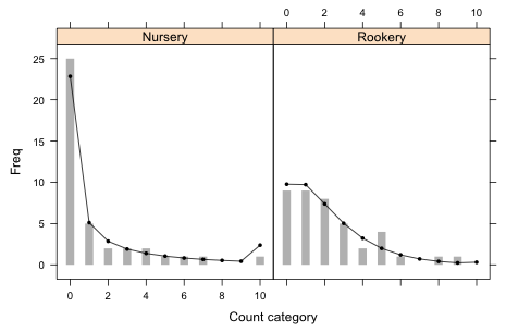
Fig. 3 Graphical fit of the separate dispersions negative binomial model
From the graph it's clear that the separate dispersions negative binomial model provides a reasonable fit to the data.
To test the goodness of fit of the separate dispersions model using the data from both fields simultaneously I use a parametric bootstrap following exactly the same protocol outlined in lecture 17 for the Poisson model. I begin by segregating the predicted probabilities by field type into the components of a list object.
$Rookery
[1] 0.244176494 0.242944651 0.184542461 0.125702509 0.080692585 0.049900146
[7] 0.030075231 0.017789536 0.010373006 0.005980645 0.007822736
The p-value of the simulation-based test is defined to be the total number of Pearson statistics that are as large or larger than the observed Pearson statistic divided by the total number of simulations.
The actual Pearson statistic is not statistically significant. The null hypothesis of the Pearson goodness of fit test is the following.
H0: fit is adequate
H1: fit is inadequate
Thus we fail to reject the null hypothesis and conclude that the fit is adequate. The analytical results are consistent with the good graphical fit we obtained in Fig. 3.
A compact collection of all the R code displayed in this document appears here.
| Jack Weiss Phone: (919) 962-5930 E-Mail: jack_weiss@unc.edu Address: Curriculum for the Environment and Ecology, Box 3275, University of North Carolina, Chapel Hill, 27599 Copyright © 2012 Last Revised--October 27, 2012 URL: https://sakai.unc.edu/access/content/group/3d1eb92e-7848-4f55-90c3-7c72a54e7e43/public/docs/lectures/lecture18.htm |