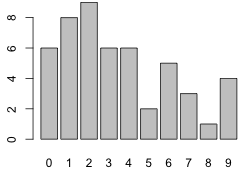
Fig. 1 Bar plot of the tabulated data
We continue with the analysis of the aphid count data set. Last time we fit a Poisson distribution to these data using maximum likelihood. Today we examine the fit of the model.
Examine the distribution of the tabulated data with a bar chart using the barplot function.
|
Fig. 1 Bar plot of the tabulated data |
Construct a function to calculate the log-likelihood of the data for a specific value of the parameter λ.
To use nlm to obtain the maximum likelihood estimate of λ, we need to change the way we're formulating the problem. Since maximizing f is equivalent to minimizing –f, we need to reformulate our objective function so that it returns the negative log-likelihood rather than the log-likelihood. I use λ = 3 as an initial guess.
I use λ = 3 as an initial guess in the call to nlm.
$estimate
[1] 3.459998
$gradient
[1] 6.571497e-08
$code
[1] 1
$iterations
[1] 4
The Poisson model that we've fit using maximum likelihood is an example of Poisson regression, which in turn is a type of generalized linear model. Generalized linear models can be fit in R using the glm function. We'll discuss generalized linear models in a more formal fashion later. For the moment think of a generalized linear model as an extension of ordinary regression to response variables that have non-normal distributions. Many of the models we've considered can be fit very simply as a generalized linear model using notation that is identical to what we used when fitting ordinary regression models. The only difference is that in a generalized linear model we need to specify a probability distribution and optionally a link function.
A link function is a function g that is applied to the mean μ of our distribution. The generalized linear model then models g(μ) as a function of predictors. If g(μ) = μ we call g the identity link. In ordinary regression when we model the mean as a linear combination of regressors we are implicitly using an identity link. While an identity link would seem to be the natural choice in all cases it is not ideal when the response variable is bounded in any way. For the Poisson distribution a log link is a better choice than an identity link and it is the default link function with the glm function and family=poisson. We can fit the Poisson distribution with the glm function as follows.
Deviance Residuals:
Min 1Q Median 3Q Max
-2.6306 -1.5612 -0.2531 1.1204 2.4753
Coefficients:
Estimate Std. Error z value Pr(>|z|)
(Intercept) 3.4600 0.2631 13.15 <2e-16 ***
---
Signif. codes: 0 ‘***’ 0.001 ‘**’ 0.01 ‘*’ 0.05 ‘.’ 0.1 ‘ ’ 1
(Dispersion parameter for poisson family taken to be 1)
Null deviance: 114.46 on 49 degrees of freedom
Residual deviance: 114.46 on 49 degrees of freedom
AIC: 250.35
Number of Fisher Scoring iterations: 3
The estimate of the intercept is the mean of the Poisson distribution and it's the same value we obtained above using the nlm function. If we fit the model without the link argument and accept the default link we are fitting the model log μ = β0. To obtain the mean of the Poisson distribution we need to exponentiate the result.
Having estimated the Poisson model we next examine how well the model fits the observed data. A good place to start is by calculating the count frequencies predicted by the model and comparing these to the observed frequencies graphically. This can be accomplished with a bar plot of the observed frequencies on which we superimpose the Poisson predictions as points connected by line segments.
I begin by calculating the expected values under a Poisson model using the estimated value of λ. I generate the Poisson probabilities for category counts 0 to 9 (matching the range of observed values we have). To obtain the expected counts I multiply these numbers by 50, the number of observations. (Note: What I'm really doing is adding up the predicted probability distributions for all 50 observations. Because each observation has the same predicted probability distribution, this is the same as multiplying that single probability distribution by 50.)
Notice that the expected values have a larger maximum than the observed values. If we sum the expected counts we find that they don't add up to 50. Equivalently, if we sum the predicted probability distribution, the probabilities don't sum to one.
That's because we're leaving off the tail probability. The Poisson distribution is unbounded above, so there is a nonzero probability of obtaining an observation with 10 or more counts. We can obtain the tail probability with the ppois function.
Alternatively we can use the lower.tail argument of ppois to calculate P(X > 9) directly.
So, we have a choice. We can create an additional category for both the observed and predicted counts, labeling it '10+' perhaps, or we can just lump P(X > 9) into the last category effectively making it represent '9 or more'.
Notice that in the second choice I calculate dpois(0:8) and then use 1-ppois(8) for the last observed category. I verify that the expected counts now sum to 50.
Either of these choices is reasonable. In what follows I use the second option. In order to add the expected counts to the bar chart I need to know the x-coordinates of the centers of the bars. You might think these are just the labels that appear below the bars, but in fact the labels shown need not correspond to the coordinate system R has used. Fortunately the coordinates used are returned by R when you assign the results of the barplot function to an object. The coordinates of the bars are the return value of the barplot function. To ensure that the expected values (which will be added to the graph with the points function) are displayed completely I will need to use the ylim argument of barplot to extend the y-axis to include the maximum expected count.
I use the barplot coordinates as the x argument of the points function. The type='o' option specifies that point symbols should be overlaid on top of line segments connecting the points.
We probably should relabel the last category to indicate that it is '9 or more' rather than just 9. The barplot function has an argument names.arg that can be used to modify the labels appearing under the bars. I also add a legend that identifies the model being fit.
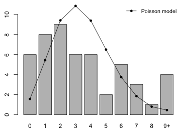
Fig. 2 Fit of the Poisson model
Based on the plot the fit doesn't look very good.
We can test the fit of the Poisson model formally with the Pearson chi-squared goodness of fit test. The Pearson chi-squared test compares the observed category frequencies to the frequencies predicted by a model (referred to as the expected frequencies) using the following formula.
where m is the number of categories. It turns out the Pearson chi-squared statistic has a chi-squared distribution.
The degrees of freedom are the number of categories, m, minus one minus the number of estimated parameters, p, used in obtaining the expected frequencies. The null hypothesis of this test is that the fit is adequate.
H0: model fits the data
H1: model does not fit the data
We should reject the null hypothesis at level α if the observed value of our test statistic exceeds the 1 – α quantile of a chi-squared distribution with m – 1 – p degrees of freedom.
Reject if ![]()
The chi-squared distribution of ![]() is an asymptotic result. For it to hold the fitted values, the expected frequencies obtained using the model, should be large. A general rule is that the expected cell counts should be 5 or larger, although with many categories Agresti (2002) notes that an expected cell frequency as small as 1 is okay as long as no more than 20% of the expected counts are less than 5. The difficulty in applying this rule when fitting a model such as the Poisson model to data is that the theoretical count distribution is infinite (although the probabilities after a certain point are essentially zero). So the 20% guideline is not well-defined.
is an asymptotic result. For it to hold the fitted values, the expected frequencies obtained using the model, should be large. A general rule is that the expected cell counts should be 5 or larger, although with many categories Agresti (2002) notes that an expected cell frequency as small as 1 is okay as long as no more than 20% of the expected counts are less than 5. The difficulty in applying this rule when fitting a model such as the Poisson model to data is that the theoretical count distribution is infinite (although the probabilities after a certain point are essentially zero). So the 20% guideline is not well-defined.
For our data quite a few of the expected counts are small. In the code below I calculate the expected frequencies, ![]() , for Poisson counts ranging from 0 to 12. From the output we see that the expected frequencies exceed 5 only for k = 1, 2, 3, 4, and 5.
, for Poisson counts ranging from 0 to 12. From the output we see that the expected frequencies exceed 5 only for k = 1, 2, 3, 4, and 5.
What to do in such a situation is not entirely clear. The standard recommendation, cited for example in Sokal and Rohlf (1995) is to pool categories. They write, p. 702, "Whenever classes with expected frequencies of less than five occur, expected and observed frequencies for those classes are generally pooled with an adjacent class to obtain a joint class with an expected frequency ![]() ." The number of categories m is thereby reduced in the degrees of freedom of the chi-squared distribution. Not everyone agrees with this. Here's a sampling from the literature.
." The number of categories m is thereby reduced in the degrees of freedom of the chi-squared distribution. Not everyone agrees with this. Here's a sampling from the literature.
My comments on this are the following.
If there are many such cases the effective result will be to dilute a significant lack of fit that may be occurring if we had just looked at the nonzero cells. Generally speaking, a chi-squared random variable to be significant must at least exceed its degrees of freedom. Each of these terms adds one degree of freedom to the test statistic. If at the same time the expected frequency is less than 1 then these terms will reduce rather than increase the lack of fit as measured by the test statistic. So I think pooling these cells in the tail makes sense.
Using 5 as a cut-off we see that we should combine the first two expected counts corresponding to k = 0 and k = 1. Turning to the right hand tail of the distribution, k = 6 is the first expected count to drop under 5. If we calculate the sum of the expected counts greater than 6 we see that these don't exceed 5 either. So we should combine all category counts for k ≥ 6
Note: ppois(6,out.pois$estimate)) = P(X ≤ 6). Therefore, 1–ppois(6,out.pois$estimate)) = P(X > 6). So, I add X = 6 to the tail too.
I next group the observed counts in exactly the same way: pool the first two, keep the next four separate, and pool the remainder. I use length(num.stems) to locate the position of the last value.
Finally I carry out the Pearson chi-squared test. It can be calculated by hand or extracted from the output of the chisq.test function. The hand calculations are as follows.
The p-value is quite small indicating a significant lack of fit. Alternatively, the critical value for our test is 9.49 and the observed value of our test statistic is 18.99, so the value of the test statistic exceeds the critical value. Therefore we reject the null hypothesis that the fit is adequate.
We can also use the chisq.test to perform the Pearson chi-square goodness of fit test. Its help screen is shown below (Fig. 3).
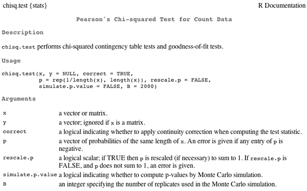
Fig. 3 Help screen for chisq.test
The entries relevant to us are x and p. The x= argument should contain the observed counts. The p= argument should contain the expected probabilities (not the expected counts). I try it for our grouped data.
data: observed
X-squared = 18.9915, df = 5, p-value = 0.001929
Observe that while the value of the test statistic is correct, the p-value is wrong as are the degrees of freedom. That's because the function doesn't know we estimated a parameter in order to obtain the expected probabilities. We can correct this by using chisq.test to obtain the Pearson statistic, but then calculate the p-value ourselves. I rerun the chi-squared test and save the result as an object in R.
The $statistic component contains the Pearson statistic. The $parameter component contains the number of categories minus one, m – 1. Because we estimated one parameter the degrees of freedom should be decreased by one more.
This matches the hand-calculation carried out above. So, we reject the null hypothesis and conclude that there is a significant lack of fit. If we supply the original unpooled data and expected probabilities to chisq.test, it warns us that the assumptions of the test are being violated.
data: num.stems
X-squared = 48.5686, df = 9, p-value = 1.999e-07
Warning message:
In chisq.test(num.stems, p = exp.pois.p) :
Chi-squared approximation may be incorrect
The chisq.test has an additional argument called simulate.p.value. Setting this argument to TRUE causes R to carry out a Monte Carlo simulation (parametric bootstrap) to obtain the p-value of the observed value of the test statistic ![]() .
This works as follows.
.
This works as follows.
The beauty of this approach is that it avoids the whole issue of whether the asymptotic chi-squared distribution is appropriate or not, because it doesn't use it! The set of simulated values defines the distribution of the ![]() statistic under the null hypothesis that the model fits the data. The issue of pooling doesn't arise, because it's not necessary. Having said that it is still necessary to combine the tail probabilities of the probability model in order to create the vector p used in the simulation. In addition there is no penalty for overfitting like there is in the parametric Pearson test where the degrees of freedom of the test statistic get reduced by p, the number of estimated parameters.
statistic under the null hypothesis that the model fits the data. The issue of pooling doesn't arise, because it's not necessary. Having said that it is still necessary to combine the tail probabilities of the probability model in order to create the vector p used in the simulation. In addition there is no penalty for overfitting like there is in the parametric Pearson test where the degrees of freedom of the test statistic get reduced by p, the number of estimated parameters.
I redo the goodness of fit test this time setting simulate.p.value=TRUE. I calculate the predicted probabilities using the Poisson model adding the tail probability to the last observed category, X = 9.
Chi-squared test for given probabilities with simulated p-value
(based on 2000 replicates)
data: num.stems
X-squared = 48.5686, df = NA, p-value = 0.0004998
Observe that the reported p-value is equal to ![]() meaning that the observed value of the test statistic was larger than any of the simulated values.
meaning that the observed value of the test statistic was larger than any of the simulated values.
With 2000 simulations our p-value is accurate to 2 or 3 decimal places. Thus the best we can say is that the true p-value is probably less than 0.001. To get a more accurate result we can increase the number of simulations by specifying our own value for the argument B. I try 9,999 simulations. I choose 9,999 so that when we include the observed value of our test statistic as one of the simulations we get the nice round number 10,000.
Chi-squared test for given probabilities with simulated p-value
(based on 9999 replicates)
data: num.stems
X-squared = 48.5686, df = NA, p-value = 3e-04
The reported p-value is equal to ![]() and tells us that there were two additional simulated values of
and tells us that there were two additional simulated values of ![]() as extreme as
as extreme as ![]() . We now have roughly 3-decimal place accuracy for our p-value and can report p < .001.
. We now have roughly 3-decimal place accuracy for our p-value and can report p < .001.
It is clear both graphically and analytically that the Poisson model does not provide an adequate fit to the aphid count data. One obvious explanation is that our model is too simple—we're assuming that a single value of λ is appropriate for all 50 observations. So a next logical step would be to allow λ to vary depending upon the value of measured predictors. Often though even after including significant predictors a Poisson regression model may still exhibit a significant lack of fit. In that case a possible solution is to switch from a Poisson distribution to a negative binomial distribution as a model for the response.
Before presenting the definition of the negative binomial distribution we need to briefly discuss the binomial distribution to which it is related. (We will explore the binomial distribution in greater detail later in the course.) In order for an experiment to be considered a binomial experiment four basic assumptions must hold.
A simple illustration of a binomial random variable is the response of a seed germination experiment. Suppose an experiment is carried out in which 100 seeds are planted in a pot and the number of seeds that germinate is recorded. Suppose this is done repeatedly for different pots that are subjected to various light regimes, burial depths, etc. Clearly the first two assumptions of the binomial model hold here.
Suppose we have five independent Bernoulli trials with the same probability p of success on each trial. If we observe the event:
![]() ,
,
i.e., three successes and two failures in the order shown, then by independence this event has probability
![]() .
.
But in a binomial experiment we don’t observe the actual sequence of outcomes, just the number of successes, in this case 3. There are many other ways to get 3 successes, just rearrange the order of S and F in the sequence SFSSF. So, the probability we have calculated here is too small. How many other distinct arrangements (permutations) of three Ss and two Fs are there?
Thus to answer the original question, the number of distinct arrangements of three Ss and two Fs is
where the last two symbols are two common notations for this quantity. Carrying out the arithmetic of this calculation we find that there are ten distinct arrangements of three Ss and two Fs. The first notation,  , is called a binomial coefficient and is read "5 choose 3". The C in the second notation denotes "combination" and thus
 ![]() is the number of combinations of five things taken three at a time. Putting this altogether, if
is the number of combinations of five things taken three at a time. Putting this altogether, if ![]() then
then
 .
.
 .
.
Here k = 0, 1, 2, … , n.
The negative binomial distribution is a popular alternative to the Poisson distribution as a model for count data (White and Bennetts, 1996; Ver Hoef and Bodeng, 1997; O'Hara and Kotze, 2010; Hilbe, 2011; Lindén and Mäntyniemi. 2011). I list some of the characteristics of the negative binomial distribution below.
The probability mass function of the negative binomial distribution comes in two distinct versions. The first one is the one that appears in every introductory probability textbook; the second is the one that appears in books and articles in ecology. Although the ecological definition is just a reparameterization of the mathematical definition, the reparameterization has a profound impact on the way the negative binomial distribution gets used. We'll begin with the mathematical definition. From an ecological standpoint the mathematical definition is rather bizarre and except for perhaps modeling the number of rejections one has to suffer before getting a manuscript submission accepted for publication, it's hard to see how this distribution is useful.
Let Xr be a negative binomial random variable with parameter p. Using the definition given above let's calculate ![]() , the probability of experiencing x failures before r successes are observed.
Note: The change in notation from k to x is deliberate. Unfortunately in a number of ecological textbooks the symbol k means something very specific for the negative binomial distribution so I don't want to use it in a generic sense here.
, the probability of experiencing x failures before r successes are observed.
Note: The change in notation from k to x is deliberate. Unfortunately in a number of ecological textbooks the symbol k means something very specific for the negative binomial distribution so I don't want to use it in a generic sense here.
If we experience x failures and r successes, then it must be the case that we had a total of x + r Bernoulli trials. Furthermore, we know that the last Bernoulli trial resulted in a success, the rth success, because that's when the experiment stops.
What we don't know is where in the first x + r – 1 Bernoulli trials the x failures and r – 1 successes occurred. Since the probability of a success is a constant p on each of these trials, we have a binomial experiment in which the number of trials is x + r – 1. Thus we have the following.
So we're done. Note: it's a nontrivial exercise to show that this is a true probability distribution, i.e.,
I'll just state the results.
The ecological definition of the negative binomial is essentially a reparameterization of the formula for the probability mass function that we just derived.
Step 1: The first step in the reparameterization is to express p in terms of the mean μ and use this expression to replace p. Using the formula for the mean of the negative binomial distribution above, I solve for p.
From which it immediately follows that
Plugging these two expressions into the formula for the probability mass function yields the following.
Step 2: This step is purely cosmetic. Replace the symbol r. There is no universal convention as to what symbol should be used as the replacement. Venables and Ripley (2002) use θ. Krebs (1999) uses k. SAS makes the substitution ![]() . I will use the symbol θ.
. I will use the symbol θ.
Step 3: Write the binomial coefficient using factorials.
Step 4: Rewrite the factorials using gamma functions. This step requires a little bit of explanation.
The gamma function is defined as follows.
![]()
Although the integrand contains two variables, x and α, x is the variable of integration and will disappear once the integral is evaluated. So the gamma function is solely a function of α. The integral defining the gamma function is called an improper integral because infinity appears as an endpoint of integration. Formally such an improper integral is defined as a limit.
Now if ![]() , but still an integer, the integral in the gamma function will be a polynomial times an exponential function. The standard approach for integrating such integrands is to use integration by parts. Integration by parts is essentially a reduction of order technique—after a finite number of steps the degree of the polynomial is reduced to 0 and the integral that remains to be computed turns out to be
, but still an integer, the integral in the gamma function will be a polynomial times an exponential function. The standard approach for integrating such integrands is to use integration by parts. Integration by parts is essentially a reduction of order technique—after a finite number of steps the degree of the polynomial is reduced to 0 and the integral that remains to be computed turns out to be ![]() (but multiplied by a number of constants). It is a simple exercise in calculus to show that
(but multiplied by a number of constants). It is a simple exercise in calculus to show that ![]() = 1.
= 1.
After the first round of integration by parts is applied to the gamma function we obtain the following.
where in the last step I recognize that the integral is just the gamma function in which α has been replaced by ![]() . This is an example of a recurrence relation; it allows us to calculate one term in a sequence using the value of a previous term. We can use this recurrence relation to build up a catalog of values for the gamma function.
. This is an example of a recurrence relation; it allows us to calculate one term in a sequence using the value of a previous term. We can use this recurrence relation to build up a catalog of values for the gamma function.
So when α is a positive integer, the gamma function is just the factorial function. But ![]() is defined for all positive α. For example, it can be shown that
is defined for all positive α. For example, it can be shown that
![]()
and then using our recurrence relation we can evaluate others, such as
![]()
Step 4 (continued): So using the gamma function we can rewrite the negative binomial probability mass function as follows.
where I've chosen to leave x! alone just to remind us that x is the value whose probability we are computing.
So what's been accomplished in all this? It would seem not very much, but that's not true. The formula we're left with bears little resemblance to the one with which we started. In particular, all reference to r, the number of successes, has been lost having been replaced by the symbol θ. Having come this far, ecologists then take the next logical step. Since the gamma function does not require integer arguments, why not let θ be any positive number? And so θ is treated solely as a fitting parameter, it's original meaning having been lost (but see below).
So, what we're left with is a pure, two-parameter distribution, i.e., ![]() , where the only restriction on μ and θ is that they are positive. With this last change, the original interpretation of the negative binomial distribution has more or less been lost and it is best perhaps to think of the negative binomial as a probability distribution that can be flexibly used to model discrete data.
, where the only restriction on μ and θ is that they are positive. With this last change, the original interpretation of the negative binomial distribution has more or less been lost and it is best perhaps to think of the negative binomial as a probability distribution that can be flexibly used to model discrete data.
It turns out that a Poisson random variable can be viewed as a special limiting case of a negative binomial random variable in which the parameter θ is allowed to become infinite. Given that there are infinitely many other choices for θ the negative binomial distribution is clearly more adaptable than the Poisson distribution for fitting data. In a sense θ is a measure of deviation from a Poisson distribution. For that reason θ is sometimes called the inverse index of aggregation (Krebs 1999)—inverse because small values of θ correspond to more clumping than is typically seen in the Poisson distribution. It is also called the size parameter (documentation for R), but most commonly of all, it is called the dispersion parameter (or overdispersion parameter).
The relationship between the negative binomial distribution and the Poisson can also be described in terms of the variances of the two distributions. To see this I express the variance of the negative binomial distribution using the parameters of the ecologist's parameterization.
Observe that the variance is quadratic in the mean. Since  , this represents a parabola opening up that crosses the μ-axis at the origin and at the point
 ![]() . θ controls how fast the parabola climbs.
. θ controls how fast the parabola climbs.
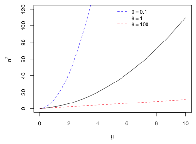 |
Fig. 4 Negative binomial mean-variance relationship as a function of θ |
As ![]() ,
, ![]() , and we have the variance of a Poisson random variable. For large θ, the parabola is very flat while for small θ the parabola is narrow. Thus θ can be used to describe a whole range of heteroscedastic behavior. Note: In the parameterization of the negative binomial distribution used by SAS,
, and we have the variance of a Poisson random variable. For large θ, the parabola is very flat while for small θ the parabola is narrow. Thus θ can be used to describe a whole range of heteroscedastic behavior. Note: In the parameterization of the negative binomial distribution used by SAS, ![]() . Thus the Poisson distribution corresponds to α = 0 and values of α > 0 correspond to overdispersion. This is perhaps the more natural parameterization.
. Thus the Poisson distribution corresponds to α = 0 and values of α > 0 correspond to overdispersion. This is perhaps the more natural parameterization.
| Jack Weiss Phone: (919) 962-5930 E-Mail: jack_weiss@unc.edu Address: Curriculum for the Environment and Ecology, Box 3275, University of North Carolina, Chapel Hill, 27599 Copyright © 2012 Last Revised--October 16, 2012 URL: https://sakai.unc.edu/access/content/group/3d1eb92e-7848-4f55-90c3-7c72a54e7e43/public/docs/lectures/lecture15.htm |