Random effects formulation
Random intercepts formulation

I reload the birds data set and create the variables needed to fit the Poisson regression models in WinBUGS and JAGS.
In the frequentist approach the transition from a Poisson separate intercepts model to a Poisson random intercepts model requires switching from glm to lmer.
Let i denote the patch and let j denote the observation from that patch (a measurement made in one of the three years). The random intercepts model can be written in two equivalent ways.
Random effects formulation |
Random intercepts formulation |
|
|
In the random effects formulation the focus is on the patch random effects, the u0i, which are assumed to have a normal distribution with mean zero. In the random intercepts formulation the focus is on the individual patch intercepts, the β0i, which are assumed to have a normal distribution with mean β0. The connection between these two formulation is that β0i = β0 + u0i. When we fit this model using lmer we automatically get both formulations. We can extract the random effects, the u0i, with the ranef function.
We obtain the random intercepts, the β0i, with the coef function.
We can also obtain the random intercepts from the random effects by adding the fixed effect estimate of the intercept, β0, to the random effects.
There is yet another way to think about this model that focuses on the structural characteristics of the data. It's called the multilevel formulation and is written as follows.
This formulation recognizes that there are quantities that vary among the observations within a patch, such as the variable year, and there are quantities that are constant within a patch but vary between patches, such as the random effects. The multilevel formulation will be especially useful when we add predictors to the model that characterize the patches.
The Bayesian version of the random intercepts model makes explicit use of the multilevel formulation. We've already seen this when we specified the separate intercepts model. As a result moving from the separate intercepts model to the random intercepts model requires only minor changes in the BUGS code. We need to replace the uninformative prior for the individual intercepts with an informative one. This change in the BUGS code is indicated below.
Separate intercepts model (model2.txt) |
Random intercepts model (model3.txt) |
| model{ for(i in 1:n) { y[i]~dpois(mu.hat[i])
log.mu[i] <- a[patch[i]] + b1*year2[i] + b2*year3[i]
mu.hat[i] <- exp(log.mu[i])
}#priors for(j in 1:J){ a[j]~dnorm(0,.000001)
}b1~dnorm(0,.000001) b2~dnorm(0,.000001) } |
model{ for(i in 1:n) { y[i]~dpois(mu.hat[i])
log.mu[i] <- a[patch[i]] + b1*year2[i] + b2*year3[i]
mu.hat[i] <- exp(log.mu[i])
}#level-2 model for(j in 1:J){ a[j]~dnorm(a.hat[j],tau.a) a.hat[j] <- mu.a } #priors mu.a~dnorm(0,.000001) tau.a <- pow(sigma.a,-2) sigma.a~dunif(0,10000) b1~dnorm(0,.000001) b2~dnorm(0,.000001) } |
In the separate intercepts model we assigned separate uninformative priors to each intercept. To a Bayesian the random intercepts model differs because each intercept is given an informative prior so that the intercepts are now modeled parameters. The notation I used for the intercepts in the BUGS code differs slightly from what I used above for the frequentist model.
The calls to WinBUGS and JAGS are shown below.
There are 106 estimated parameters, far too many to squeeze the trace plots of the Markov chains into a single graphics window. I plot them instead 16 per panel. The last set of trajectories is shown in Fig. 1. All of the chains appear to be mixing well.
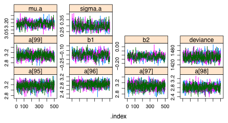 |
| Fig. 1 Trace plots of individual Markov chains from WinBUGS. |
Checking the summary object we find that all of the Rhats are less than 1.1 and the effective sample sizes are large.
The means of the Bayesian posterior distributions for the population intercept, the regression coefficients, and the standard deviation of the random effects are all very close to the frequentist MLEs. (In the notation I've used mu.a corresponds to the frequentist intercept β0.)
The frequentist predictions of the random intercepts are also close to the Bayesian posterior means. (Only the first 12 of these are shown below.)
We can also fit the random effects formulation of the random intercepts model as a Bayesian model. The BUGS code for the random intercepts version and the random effects version of the model are shown below with the differences highlighted.
Random intercepts version (model3.txt) |
Random effects version (model3a.txt) |
| model{ for(i in 1:n) { y[i]~dpois(mu.hat[i])
log.mu[i] <- a[patch[i]] + b1*year2[i] + b2*year3[i]
mu.hat[i] <- exp(log.mu[i])
}#level-2 model for(j in 1:J){ a[j]~dnorm(mu.a,tau.a) } #priors mu.a~dnorm(0,.000001) tau.a <- pow(sigma.a,-2) sigma.a~dunif(0,10000) b1~dnorm(0,.000001) b2~dnorm(0,.000001) } |
model{ for(i in 1:n) { y[i]~dpois(mu.hat[i])
log.mu[i] <- a[patch[i]] + b1*year2[i] + b2*year3[i]
mu.hat[i] <- exp(log.mu[i])
}#level-2 model for(j in 1:J){ a[j] <- mu.a + u0[j] u0[j]~dnorm(0,tau.a) } #priors mu.a~dnorm(0,.000001) tau.a <- pow(sigma.a,-2) sigma.a~dunif(0,10000) b1~dnorm(0,.000001) b2~dnorm(0,.000001) } |
To run the random effects version of the model requires changing the initial values and the returned parameters.
I compare the frequentist predictions of the random effects with the Bayesian means. Although there are some differences, the results are similar.
We've already seen that the lmer function does not report a log-likelihood for Poisson models that is comparable to what is reported for other Poisson models (lecture 22). Even if we adjust for this and also take into account the difference between ![]() and
and ![]() in the Bayesian formulation, the Bayesian and frequentist deviances with mixed effects models are not directly comparable. In the Bayesian calculations the reported deviance is based on the joint likelihood of the data and the random effects, an expression we would write as follows.
in the Bayesian formulation, the Bayesian and frequentist deviances with mixed effects models are not directly comparable. In the Bayesian calculations the reported deviance is based on the joint likelihood of the data and the random effects, an expression we would write as follows.
In the frequentist approach the reported log-likelihood is based on the marginal likelihood of y in which the random effects have been integrated out. These two likelihoods are not the same nor do they contain the same information about model fit.
So far all the random intercepts models for richness that we've considered have included a single predictor, year, whose value varied across observations. The other variable patch that appeared in the model played a role not as a predictor but as a structural variable. Patch describes how the data are organized, the fact that separate annual observations were made on the same patch yielding a hierarchical data set. The layers of the hierarchy are referred to as levels and so the birds data set is also a 2-level data set. Level 1 corresponds to the individual annual observations; level 2 corresponds to the patch observations while the patch itself is referred to as a level-2 unit. The variable year is a level-1 predictor. This break-down resembles the split plot design discussed in lecture 10 where we had split plot (level 1) units as well as whole plot (level 2) units.
The next complication is to include level-2 predictors in the model. For the birds data set a level-2 predictor is a patch characteristic. All observations made on the same patch will necessarily share the same value of a level-2 predictor. The distinction between level-1 and level-2 predictors is important because the level of a predictor determines how one should measure background variability for use in a statistical test of the predictor's effect on the response. With level-1 predictors measurements from the same patch or from different patches all count as suitable replicates (although there are issues of correlation that need to be addressed), but with a level-2 predictor only measurements made on different patches should contribute to assessing the effect of that predictor. Taking repeated measurements of the same level-2 unit and treating them as if they were true replicates of the effect of the level-2 predictor is called pseudo-replication.
In the birds data set the variables landscape and area can serve as level-2 predictors. Landscape classifies the land use type for each patch and area records the size of each patch. Because they are level-2 predictors they have the same value for all observations made on the same patch. When we fit the model using the lmer function we just include level-2 predictors as ordinary predictors; lmer figures out the appropriate way to deal with them based on their variability in the data set. Previously we used log(area) as the regressor rather than area.
Contrary to our experience with lmer, a formal distinction between level-1 and level-2 predictors must be made when fitting a Bayesian model. As we've seen a level-1 predictor has a different value for each observation while a level-2 predictor has a different value for each level-2 unit, here the patch. In the Bayesian model the data for the level-2 regressors must consist of only one observation per patch. To accomplish this we use the tapply function to select one value of log(area) and landscape from each patch. The generic function function(x) x[1] will accomplish this. The following line of code extracts one value of log(area) from each patch.
If we examine the class of the variable L.area that tapply has created we discover that it is of type "array".
While JAGS has no problem with data in this format, WinBUGS does. WinBUGS accepts only numeric data. We can change the class of L.area to type "numeric" by using either the as.vector function or the as.numeric function on the output of tapply.
The data are now in the format that WinBUGS requires, but the display of values reveals another problem. There is a missing value for L.area. Using the output above from when L.area was of class "array" we see that this missing value corresponds to a patch labeled "Ref1h". When we try to list its data in the current data frame we find that this patch doesn't exist.
On the other hand patch 'Ref1h' is present in the original data frame where it has a non-missing value for area.
Notice that this patch has missing values for richness S in all three years and as a result all of its observations were deleted when we created the birds.short data frame. The levels of a factor are defined when the factor is first created and these levels are then inherited by all subsets of the original data frame, regardless of how many levels of the factor are actually represented in the subset. The way around this is to use the factor function again to redefine the factor variable so that it will have only the unique levels that are present in the current data frame. It's worth noting that the as.factor function, which a lot of people in this class like to use, does not work here. The as.factor function will only create a factor from a variable that is not a factor. If it is already a factor it just leaves it alone.
We need to create a level-2 version of the landscape variable too.
The factor levels of the landscape variable have been automatically converted to numeric values by tapply. For the regression model we need to create three indicator variables that indicate the 2nd, 3rd, and 4th levels of landscape.
Level-2 predictors should appear in the level-2 part of the BUGS model. So in the BUGS code for the random intercepts model the level-2 predictors should appear as predictors in the model for a.hat, the individual patch mean. The table below shows the basic random intercepts model in the left panel and indicates in the right panel where the level-2 predictors should be placed in the model. I save the model as model4.txt.
Random intercepts model |
Random intercepts model with level-2 predictors |
| model{ for(i in 1:n) { y[i]~dpois(mu.hat[i])
log.mu[i] <- a[patch[i]] + b1*year2[i] + b2*year3[i]
mu.hat[i] <- exp(log.mu[i])
}#level-2 model for(j in 1:J){ a[j]~dnorm(a.hat[j],tau.a) a.hat[j]<-mu.a } b1~dnorm(0,.000001) b2~dnorm(0,.000001) mu.a~dnorm(0,.000001) tau.a<-pow(sigma.a,-2) sigma.a~dunif(0,10000) } |
model{ for(i in 1:n) { y[i]~dpois(mu.hat[i])
log.mu[i] <- a[patch[i]] + b1*year2[i] + b2*year3[i]
mu.hat[i] <- exp(log.mu[i])
}
#level-2 model
for(j in 1:J){
a[j]~dnorm(a.hat[j],tau.a)
a.hat[j]<-mu.a + g1*L.area[j] + g2*Lscape2[j]
+ g3*Lscape3[j] + g4*Lscape4[j]
}g1~dnorm(0,.000001) g2~dnorm(0,.000001) g3~dnorm(0,.000001) g4~dnorm(0,.000001) b1~dnorm(0,.000001) b2~dnorm(0,.000001) mu.a~dnorm(0,.000001) tau.a<-pow(sigma.a,-2) sigma.a~dunif(0,10000) } |
The new variables are added to the list of data in the bird.data and bird.parms arguments and additional initial values are included in the bird.inits argument.
These results compare favorably with the frequentist results obtained above. The largest difference occurs in the standard deviation of the level-2 random effects, sigma.a, labeled (intercept) in the VarCorr output.
| Predictor | Parameter |
Bayesian estimate
(mean of posterior distribution) |
Frequentist estimate |
| Intercept | β0 |
3.062 |
3.066 |
| Year 2 | β1 |
–0.131 |
–0.130 |
| Year 3 | β2 |
–0.108 |
–0.109 |
| log(Area) | γ1 |
0.223 |
0.222 |
| Bauxite | γ2 |
–0.228 |
–0.229 |
| Forest | γ3 |
–0.065 |
–0.067 |
| Urban | γ4 |
–0.266 |
–0.267 |
τ |
0.148 |
0.138 |
One of the major attractions of Bayesian estimation is the ease with which it is possible to obtain interval estimates for auxiliary parameters that are functions of parameters in the model. To obtain the posterior distribution of an auxiliary parameter defined by a function we just apply that function to the posterior distributions of the parameters that appear in its formula. We can do this either by defining the auxiliary parameters explicitly in the model or by calculating them after the model is fit.
Suppose we want to obtain interval estimates of the mean bird richness in the year 2005 for patches with area = 1 separately for each of the four landscape types. The fitted model for the log mean is the following.
the desired means are the following.
We can add these calculations to the BUGS program file.
Model with landscape means (model4.txt) |
model{
for(i in 1:n) {
y[i]~dpois(mu.hat[i])
log.mu[i] <- a[patch[i]] + b1*year2[i] + b2*year3[i]
mu.hat[i] <- exp(log.mu[i])
}
#level-2 model
for(j in 1:J){
a[j]~dnorm(a.hat[j],tau.a)
a.hat[j] <- mu.a + g1*L.area[j] + g2*Lscape2[j]
+ g3*Lscape3[j] + g4*Lscape4[j]
}
g1~dnorm(0,.000001)
g2~dnorm(0,.000001)
g3~dnorm(0,.000001)
g4~dnorm(0,.000001)
b1~dnorm(0,.000001)
b2~dnorm(0,.000001)
mu.a~dnorm(0,.000001)
tau.a <- pow(sigma.a,-2)
sigma.a~dunif(0,10000)
mean1 <- exp(mu.a)
mean2 <- exp(mu.a + g2)
mean3 <- exp(mu.a + g3)
mean4 <- exp(mu.a + g4)
}
|
We can refit this model from scratch, or better yet, we can restart the model we previously estimated using the last values of the Markov chains of the sampled parameters as the new initial values. These are stored in the $last.values component of the bugs object and can be used instead of bird.inits as the initial values. The other change is that we need to add the means to the bird.parms object so that samples of their posterior distributions are returned to us.
Given that we already have samples from the posterior distributions of all the parameters that are needed for the calculations of the means, we don't actually need to fit the model again. Instead we can perform the arithmetic on the vectors of samples and then obtain the interval estimates from the results. I first calculate the posterior distributions of the means and then assemble the results in a matrix in the order "agricultural", "bauxite", "forest", and "urban".
The percentile 95% credible intervals can be calculated in the usual fashion.
Or we can convert the matrix to an mcmc object and calculate the HPD intervals.
WinBUGS and JAGS and for that matter Bayesians in general use the term deviance to mean –2 times the log-likelihood of the model.
deviance = –2 × log-likelihood
This differs from the classical definition of deviance used in generalized linear models where the deviance (scaled) was defined as twice the difference in the log-likelihoods between the current model and the so-called saturated model—a model in which there is a separate parameter estimated for every observation. The deviance defined in this way can be used as a goodness-of-fit statistic for Poisson or grouped binary data, but only when the expected cell counts meet certain minimum cell-size criteria.
Now in certain circumstances the log-likelihood of the saturated model turns out to be zero and for these cases the Bayesian and classical definitions of the deviance are the same. One example is with binary data in which the response is assumed to have a Bernoulli distribution. For most other probability models the saturated model will contribute a nonzero term to the classical definition of the deviance and as a result the classical definition and the Bayesian definition will not agree. Unfortunately the Bayesian use of the term deviance, in which the contribution of the saturated model to the deviance is ignored, is now well-established in the literature. As a result use of the term "deviance" is ambiguous.
We saw in lecture 24 that for a Poisson fixed effects models, the estimated log-likelihood returned by WinBUGS based on ![]() is approximately the same as the log-likelihood returned by frequentist software. This will generally be the case when the models in question involve only fixed effects (although differences can arise due to the way variances are estimated by maximum likelihood). When random effects are thrown into the mix, the situation changes and the log-likelihoods returned are no longer the same.
is approximately the same as the log-likelihood returned by frequentist software. This will generally be the case when the models in question involve only fixed effects (although differences can arise due to the way variances are estimated by maximum likelihood). When random effects are thrown into the mix, the situation changes and the log-likelihoods returned are no longer the same.
In hierarchical models with both fixed and random effects, the log-likelihoods estimated by Bayesian and frequentist software can differ markedly. This occurs because Bayesians and frequentists are no longer estimating the same quantity. As was explained in lecture 22, frequentists work with what is called the marginal likelihood, the likelihood obtained after integrating out the random effects from the joint likelihood of the parameters and the random effects. Bayesians instead work directly with the joint likelihood and treat the individual random effects as parameters to be estimated. This poses an interesting conundrum. We've argued that one of the advantages that random effects models have over fixed effects (separate regressions) models is that they are more parsimonious and do not overfit models to data. But if in the Bayesian approach the random effects are estimated directly as part of fitting the model, then where is the parsimony?
Bayesians address the issue of parsimony with a model characteristic they call the effective number of estimated parameters, or pD. The term "effective" is used because unlike the parameters obtained in a separate regressions model, the parameters in a Bayesian mixed effects model are subject to constraints.
These ideas get used formally in the Bayesian formulation of model complexity. If model parameters are constrained, either through their priors or because they arise from a common distribution as is the case with random effects, then the actual number of parameters in the model is not a true reflection of model complexity. Instead we need to know the effective number of parameters, pD, a correction to the actual number of parameters that takes into account their mutual constraints. Bayesians then use pD to calculate DIC, the Bayesian version of the information-theoretic model selection statistic AIC.
Recall that AIC is a measure of relative model complexity in that it estimates expected relative Kullback-Leibler information. In a simplistic sense AIC can be thought of as penalized log-likelihood in which increases in log-likelihood that are achieved by increasing a model's complexity are penalized according to the number of extra parameters that have been added to the model. Using Bayesian notation AIC can be written as follows.
![]()
Here ![]() is the deviance calculated at the modes of the posterior distributions of all parameters in the model and K is number of parameters estimated in fitting the model. Bayesians replace AIC with DIC that is estimated as follows.
is the deviance calculated at the modes of the posterior distributions of all parameters in the model and K is number of parameters estimated in fitting the model. Bayesians replace AIC with DIC that is estimated as follows.
![]()
where ![]() is the deviance calculated at the means of the individual parameter posterior distributions and pD is as defined above. DIC is an acronym for "deviance information criterion". All of this begs the question of how model complexity, pD, in Bayesian models is determined. There are a number of definitions but the most popular one is due to Spiegelhalter et al. (2002). (David Spiegelhalter is one of the primary developers of the WinBUGS software.) Their definition is
is the deviance calculated at the means of the individual parameter posterior distributions and pD is as defined above. DIC is an acronym for "deviance information criterion". All of this begs the question of how model complexity, pD, in Bayesian models is determined. There are a number of definitions but the most popular one is due to Spiegelhalter et al. (2002). (David Spiegelhalter is one of the primary developers of the WinBUGS software.) Their definition is
![]()
where ![]() is the mean of posterior distribution of the deviance.
is the mean of posterior distribution of the deviance.
Their rationale for this definition is as follows. Each MCMC sample of D is calculated using the current values of the parameters in the Markov chains that are samples from their respective posterior distributions. Because at any given iteration these values are not likely to be at the modes, or means for that matter, of their respective posterior distributions, the calculated log-likelihood obtained from D will be less than its maximum possible value. Said differently the deviance obtained in this fashion will be larger than ![]() . The mean of all the deviance values in the sample,
. The mean of all the deviance values in the sample, ![]() , will also exceed
, will also exceed ![]() and hence pD defined by the above formula should be non-negative.
and hence pD defined by the above formula should be non-negative.
When there are more constraints on the individual parameters, D will have less room to vary. Thus the individual values of D will on average be closer to ![]() . When there are fewer constraints on the parameters, values of D can vary more and will typically be further from
. When there are fewer constraints on the parameters, values of D can vary more and will typically be further from ![]() . When there are no constraints at all on the parameters (a separate intercepts regressions model with uninformative priors) pD assumes its largest possible value which turns out to be equal to K, the number of parameters in the frequentist definition of AIC. As the number and strength of the constraints is increased, pD decreases from this maximum value. While additional steps are needed to make this argument rigorous, this is essentially the motivation for the Bayesian definition of DIC. Additional information can be found in McCarthy (2007).
. When there are no constraints at all on the parameters (a separate intercepts regressions model with uninformative priors) pD assumes its largest possible value which turns out to be equal to K, the number of parameters in the frequentist definition of AIC. As the number and strength of the constraints is increased, pD decreases from this maximum value. While additional steps are needed to make this argument rigorous, this is essentially the motivation for the Bayesian definition of DIC. Additional information can be found in McCarthy (2007).
The bugs function returns pD as a model component.
In the current model there are seven regression parameters and one variance term for a total of eight fixed effects parameters. This is the number of parameters used by frequentists to calculate AIC.
Yet WinBUGS has determined there are 59.039 effective parameters, roughly 51 more than the number of fixed effects parameters. Random effects in Bayesian models are treated as modeled parameters, but because they are constrained to come from a common distribution they are not free to vary independently of each other. So, even though there are 101 random intercepts in the model,
due to the constraints WinBUGS counts them as being effectively equivalent to 51 free parameters. WinBUGS also returns DIC as a model component.
Although WinBUGS does not return ![]() it does return
it does return ![]() . This is enough for us to calculate DIC ourselves because
. This is enough for us to calculate DIC ourselves because ![]() is not needed as the following algebra shows.
is not needed as the following algebra shows.
![]()
Plugging this expression for ![]() into the DIC formula yields the following alternative formula.
into the DIC formula yields the following alternative formula.
![]()
Using this we find
which agrees with the reported DIC. Interestingly JAGS reports completely different values for pD and DIC than does WinBUGS.
The mean deviance ![]() reported by JAGS is in agreement with the value reported by WinBUGS.
reported by JAGS is in agreement with the value reported by WinBUGS.
and using the alternative formula for DIC we obtain the value reported by JAGS.
Thus the difference between JAGS and WinBUGS is in how pD is calculated. An explanation of what JAGS is doing can be found here.
Because DIC and AIC in mixed effects models work with different log-likelihoods, they are not directly comparable. Whether AIC is an appropriate way to compare mixed effects models is a matter of debate. An alternative definition of AIC has been proposed by Vaida and Blanchard (2005) for mixed effects models. They call their version conditional AIC and it is essentially a frequentist formulation of DIC. They promote the use of conditional AIC for model comparison when the random effects are of primary interest and not merely nuisance parameters. At present it is not known how to calculate conditional AIC except in a few special cases.
A compact collection of all the R code displayed in this document appears here.
| Jack Weiss Phone: (919) 962-5930 E-Mail: jack_weiss@unc.edu Address: Curriculum for the Environment and Ecology, Box 3275, University of North Carolina, Chapel Hill, 27599 Copyright © 2012 Last Revised--November 23, 2012 URL: https://sakai.unc.edu/access/content/group/3d1eb92e-7848-4f55-90c3-7c72a54e7e43/public/docs/lectures/lecture25.htm |