(a) 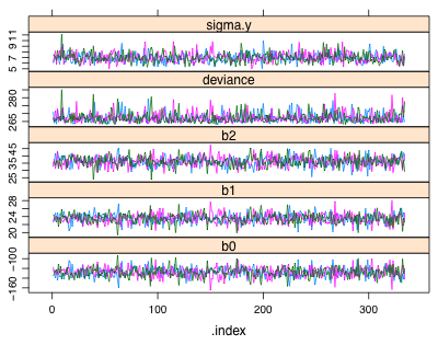
(b) 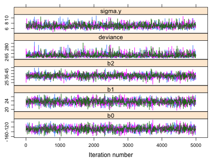
I refit the frequentist and Bayesian analysis of covariance models we worked with in lecture 23. For this I use the BUGS model definition file ipomodel.txt from lecture 23.
Using the argument debug=T of the bugs function causes the WinBUGS program to pause after the model is fit allowing us to inspect the graphs and diagnostics that WinBUGS has produced before the program shuts down and the numerical results are returned to R. It is not possible to do this with the jags function because JAGS is not a stand-alone application. Trace plots of the Markov chains have to be generated in R.
When the arm and R2jags packages are loaded, the coda package is also loaded into memory. The coda package provides a number of tools and diagnostics for Bayesian models. To use them we have to first create an mcmc object. For a bugs object we do this with the as.mcmc.list function while for a jags object we use the as.mcmc function.
To obtain trace plots of the individual Markov chains we can use the xyplot function from lattice on the mcmc object that has been created. Fig. 1a shows the output from bugs while Fig. 1b shows the output from jags.
(a) |
(b) |
| Fig. 1 Trace plots of individual Markov chains from (a) WinBUGS and (b) JAGS. |
Each chain (denoted by a different color) derives from a different random start of the MCMC algorithm. The displayed trajectories trace the sampled values in the order they were obtained for each chain. (Compare this with the discussion of the toy example of the Metropolis algorithm given in lecture 23.) By default both jags and bugs are set up to treat the first half of the iterates as part of the the burn-in period. So the first 5,000 iterations of this run of 10,000 are discarded and only the values from the second half of the run are saved. (This can be changed by specifying a value for the n.burnin argument.)
Both jags and bugs have thinned the chains to reduce memory use and to decrease the correlation between the sampled observations. The default thinning rate for WinBUGS is max(1, floor(n.chains*(n.iter-n.burnin)/1000). The n.thin argument can be used to override this default. With n.chains = 3, n.iter = 10000, and n.burnin = 5000, the thinning rate is 15. Thus only every 15th simulation value is saved. With 3 chains this means BUGS will return 1002 (3 times 334) samples that hopefully, if convergence has been attained, will be samples from the posterior distributions of each parameter. JAGS apparently thins things on a per chain basis so that 1000 observations remain in each chain. As a result the thinning rate here is only 5. Thus JAGS returns three times as many observations as does WinBUGS. That's why the trace plots from JAGS look like they have more observations. They do!
Another difference in the plots is how the x-axis is labeled. The x-axis for WinBUGS output denotes the actual position of the sampled observation in the thinned chain. For JAGS the x-axis denotes the original index location of the sampled observation in the unthinned chain.
Using the trace plots we can assess whether the chains have converged to the posterior distribution and whether we've obtained a random sample from that distribution. From Fig. 1 we can conclude the following.
The summary component returned by bugs and jags (for jags the summary component is contained in the BUGSoutput component) contains two useful diagnostics for assessing mixing and convergence of the individual Markov chains: Rhat and n.eff.
Rhat is the mixing index. Numerically it is the square root of the variance of the mixture of all the chains divided by the average within-chain variance. If the chains are mixing these values should be roughly the same yielding a ratio of approximately 1. A useful decision rule is to stop when all the reported Rhat values for the different parameters are less than 1.10. With small models such as this one the Rhat values can be examined individually. For larger models determining the maximum reported Rhat is a more practical option. Because the largest returned value of Rhat for the current model is less than 1.10 we have evidence the chains are mixing well.
The statistic n.eff is a crude measure that tries to account for the correlations between the successive values of the thinned Markov chain to provide a measure of effective sample size. Due to correlation the effective sample size will tend to be smaller than the actual number of simulations. The effective sample size is calculated indirectly by comparing two different measures of variability and should not be taken too seriously. Still, we want this number to be relatively large particularly for the parameters that are of special interest to us, i.e., the parameters for which we need an interval estimate. Extremely small values of n.eff should be worrisome. For both the JAGS and WinBUGS runs the smallest reported effective sample size turns out to be quite large.
The densityplot function of lattice can be used to display kernel density estimates (smoothed histograms) of the frequency distributions of the sampled posterior distributions obtained by MCMC. The default display when densityplot is applied to the mcmc objects we've created is to produce a separate density plot for each chain.
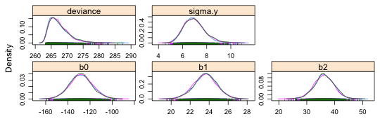 |
Fig. 2 Posterior densities for individual parameters and individual Markov chains |
In order to get a single density estimate for each parameter we need to combine the individual chains. There are two ways to do this.
The mcmc object created from a bugs or jags object is a list of matrices. We can rbind the individual list elements together and plot the result.
This can be done more efficiently with the do.call function of R.
The do.call function resembles sapply in that it can be used to apply a function to a list of elements. Unlike sapply which applies a function separately to each component of the list, do.call applies the function to all list components simultaneously. Thus in the above call we end up rbinding the list components of bugsfit.mcmc together. The result is a matrix and no longer an mcmc object so we need to use the as.mcmc function on the result. (We use as.mcmc here rather than as.mcmc.list because the object is not a list.)
There's no reason to display the posterior distribution of the deviance, so I redo the plot but this time specify only the columns that I want displayed (Fig. 3). At the bottom of each density plot is a rug plot of the data. The density plot summarizes our posterior beliefs about the true values of the parameters indicating which values are more likely and which values are less likely.
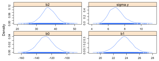 |
Fig. 3 Estimated posterior densities for individual parameters |
A simpler way of producing a single density plot for each parameter is to work with the sims.matrix component of the bugs object. We first need to convert it to an mcmc object with the as.mcmc function after which we can plot the result.
The $summary component of the bugs object contains some representative quantiles of the posterior distribution for each parameter. Using these values we can construct 95% percentile credible intervals for the parameters.
We can also calculate these quantiles using the $sims.matrix component of the bugs object. To get them in this fashion we just use the quantile function.
To obtain credible intervals for more than one parameter at a time we can use the sapply function.
To compare these results to the frequentist's 95% confidence intervals, we can apply the confint function to the corresponding lm model object, out2. The two sets of intervals are similar.
An alternative way to calculate Bayesian credible intervals is as an HPD (highest posterior density) interval, also known as an HDI. The HDI contains those x-values that have highest believability. Let f(x) denote the posterior density of a parameter as estimated by MCMC. To calculate the HDI we need to find a value W such that integrating the posterior density over x where f(x) > W yields a probability = 0.95.
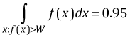
Generally the HDI and percentile intervals are similar, but Fig. 4 illustrates a case where they are quite different. The estimated posterior distribution of θ is bimodal. As a result, choosing the most probable values of θ such that the probability sums to 0.95 has yielded two disjoint intervals that together define the HPD interval. The percentile interval on the other hand is a single interval that also includes a region of fairly improbable values of θ, the interval around 3 that lies between the two modes of the posterior distribution.
 |
| Fig. 4 Contrasting HPD credible intervals and percentile credible intervals for a posterior distribution that is bimodal. (R code for Fig. 4) |
The HPDinterval function can be used to extract HPD intervals from an mcmc object. Like densityplot, HPDinterval when applied to an mcmc object created from a bugs or jags object will return HPD intervals separately for each chain. To obtain single HPD intervals using the data from all three chains simultaneously we can create the mcmc object from the sims.matrix component.
The results are quite similar to the percentile intervals calculated previously.
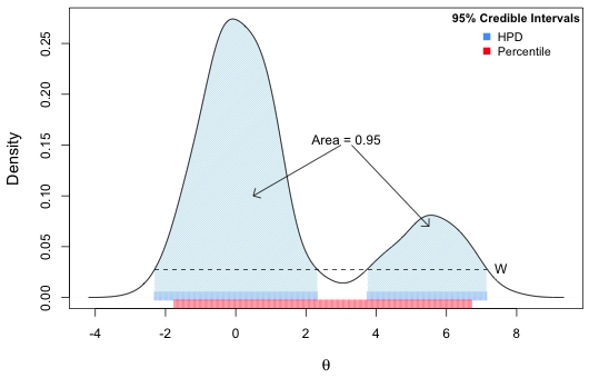
With an entire posterior distribution at our disposal we have to choose what we want to call the Bayesian point estimate. Obvious choices are the mean or the median of the posterior distribution. For symmetrical posterior distributions these should be fairly similar. The frequentist maximum likelihood estimate is the value of the parameter that maximizes the likelihood, the parameter value that makes the data we obtained most likely. With an uninformative prior, the posterior distribution should be proportional to the likelihood in which case the maximum likelihood estimate should correspond to the mode of the posterior distribution.
Fig. 5 displays a kernel density estimate (smoothed histogram) of the posterior distribution of the intercept, b0, using the samples of the posterior distribution contained in the $sims.matrix component. Indicated on the graph are the locations of the maximum likelihood estimate (frequentist estimate from lm) as well as the mean, median, and mode of the estimated posterior distribution (Bayesian). Observe that all the estimates are very close to each other.
 |
| Fig. 5 Posterior distribution of the intercept |
We saw an example in lecture 23 where presumably uninformative priors turned out to be too informative and managed to affect the posterior estimates we obtained. While we might therefore be tempted to choose priors that are very uninformative, priors that allow parameters to have too wide a range can lead to computational instability. In WinBUGS this results in an error message such as "cannot bracket slice for node...." indicating that the current prior is too diffuse. A good general strategy is to rescale the variables in the model so that all the regression parameters have the same limited range. A reasonable rule is to rescale things so that parameter values lie in the interval –10 to 10. When things are scaled in this way beforehand, the same uninformative priors will work for every model and no further adjustments need to be made to the priors.
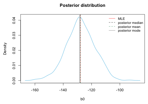
Without prior information about a regression parameter, the usual approach is to assume that a regression parameter has a normal distribution with a mean of zero (representing no relationship with the response) and a very large variance. This choice yields a prior distribution that is roughly flat over its likely range and leaves the regression parameter essentially unrestricted. Because the normal distribution in the BUGS language is parameterized in terms of precision rather than variance, a large variance is obtained by specifying a very small precision. Fig. 6 shows four normal priors with decreasing levels of precision (increasing variance). Notice that as the precision is decreased each normal distribution is flatter than the one before. On the scale of the most precise normal prior, dnorm(0, .01), the least precise normal prior, dnorm(0, .00001), appears to be essentially flat.
 |
| Fig. 6 The effect of varying the precision parameter of normal priors |
The following line is commented out in the BUGS program file we used in lecture 23.
tau.y~dgamma(.001,.001)
This gives an "uninformative" prior for the precision parameter of a normal distribution and is the prior that typically appears in textbooks on Bayesian modeling. In general if Y ~ dgamma(a,b) then Y has mean![]() and variance
and variance ![]() . The two parameters of the gamma distribution used in the BUGS parameterization are referred to as the shape and rate parameters in the R parameterization. Fig. 7 illustrates how changing these two parameters affects the shape of the gamma distribution.
. The two parameters of the gamma distribution used in the BUGS parameterization are referred to as the shape and rate parameters in the R parameterization. Fig. 7 illustrates how changing these two parameters affects the shape of the gamma distribution.
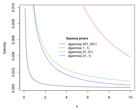 |
| Fig. 7 The effect of varying parameter values on the gamma prior |
The prior dgamma(.001,.001) is a gamma distribution with a mean of 1 and a variance of 1000. From the graph this resembles a classic dust bunny distribution (McCune & Grace 2002). Nearly all of the weight is placed at zero but because of the large variance, large values are also possible. Without the large spike at zero, the prior is essentially flat. Because this is a prior for a precision parameter, a large weight at zero is not considered a problem. In using such a prior for the precision we're saying that we have no information about the parameter that has this precision.
The primary rationale for using a gamma prior is that it is a conjugate prior for the precision in a normal model with a known mean. (Technically when the normal priors for the regression coefficients are independent of the gamma prior for the precision, as they are here, we call them conditionally conjugate or semi-conjugate priors for the normal mean and precision.) Using a conjugate prior yields a posterior distribution of known form. While historically this was essential for getting estimates analytically, with MCMC it is no longer considered necessary. In the BUGS program of lecture 23 instead of modeling the precision tau.y directly we chose instead to place a uniform prior on sigma.y, the standard deviation. This is also the approach taken by Gelman & Hill (2006) and Jackman (2009).
tau.y <- pow(sigma.y,-2)
sigma.y~dunif(0,10000)
In BUGS models gamma priors for precisions tend to cause numerical problems more often than do uniform priors for standard deviations. Furthermore the spike at the origin can make it difficult to get variance estimates in some of the multilevel problems we'll be considering later. A gamma prior that is flat over most of its distribution but is quite informative around zero causes problems if the true value of the precision parameter is actually close to zero. Consequently I will rarely use a gamma prior for the precision in this course.
We next revisit a data set we analyzed in lecture 22. This is the Jamaican birds data set in which the goal was to determine if bird richness varied by landscape type, in particular whether areas that had been subjected to bauxite mining exhibited lower bird richness. The response variable S is a species count. The counts are far removed from zero and have a modest range so we chose to use a Poisson distribution for the response. Species richness counts were obtained from the same patch in multiple years so this is a repeated measures data set. Patches also varied widely in their area so we included log(area) as a covariate. Our final model included a categorical predictor for year, log(area) as a covariate, and a landscape categorical predictor that classified each patch. To account for the repeated measures we included patch random effects that linked together the observations made on the same patch. The final model was a generalized linear mixed effects model that we fit using the lmer function of the lme4 package. Our goal today is to reproduce those results using Bayesian methods.
I start by fitting a Poisson regression model that ignores the inherent structure of these data. This is sometimes referred to as the complete pooling model. I begin with a model that includes categorical year as the only predictor. The Poisson distribution in BUGS is specified with dpois, the same name as the Poisson probability mass function of R. Consistent with the frequentist approach I use a log link, thus I set the linear predictor equal to the log mean. Therefore to obtain the mean of the Poisson distribution I have to exponentiate the linear predictor.
Complete pooling model (model1.txt) |
model{
for(i in 1:n) {
y[i]~dpois(mu.hat[i])
# log link
logmu.hat[i] <- a + b1*year2[i] + b2*year3[i]
mu.hat[i] <- exp(logmu.hat[i])
}
a~dnorm(0,.000001)
b1~dnorm(0,.000001)
b2~dnorm(0,.000001)
} |
I create the variables and objects needed to fit the model.
The deviance statistic reported in the summary table is not the residual deviance or null deviance that we've seen reported in the output of the glm function. It is just –2 × log-likelihood of the model. If we compare this to –2 × log-likelihood for the frequentist model we see there is a slight discrepancy.
The frequentist value is three less than the Bayesian mean deviance. The deviance reported in the BUGS summary table is the average of the separate deviance values from all of the returned Markov chain samples. It is the mean of the posterior distribution of the deviance. This is what the Bayesians denote as ![]() . The frequentist value on the other hand is the deviance (–2 × log-likelihood) calculated at the maximum likelihood estimates of the parameters. A Bayesian would approximate the frequentist value by evaluating –2 × log-likelihood at the mean of the posterior distributions of the three parameters in the model, a statistic that Bayesians denote
. The frequentist value on the other hand is the deviance (–2 × log-likelihood) calculated at the maximum likelihood estimates of the parameters. A Bayesian would approximate the frequentist value by evaluating –2 × log-likelihood at the mean of the posterior distributions of the three parameters in the model, a statistic that Bayesians denote ![]() . Because the reported posterior means are all close to the frequentist maximum likelihood estimates,
. Because the reported posterior means are all close to the frequentist maximum likelihood estimates, ![]() will be approximately the same as the frequentist value of –2 × log-likelihood. We can verify this by obtaining the means of the posterior distributions of the parameters and then calculating the Poisson log-likelihood.
will be approximately the same as the frequentist value of –2 × log-likelihood. We can verify this by obtaining the means of the posterior distributions of the parameters and then calculating the Poisson log-likelihood.
Bayesians calculate the effective number of parameters in the model by subtracting these two quantities.
![]() .
.
As we've seen ![]() is three less than
is three less than ![]() and this does equal the number of model parameters. Bayesians calculate a statistic DIC (deviance information criterion) that is analogous to AIC. It is defined as follows.
and this does equal the number of model parameters. Bayesians calculate a statistic DIC (deviance information criterion) that is analogous to AIC. It is defined as follows.
![]()
It's returned as part of the output from the bugs function and is approximately the same as AIC here.
Generally speaking the separate intercepts model is usually not interesting because it severely overfits the data. From a Bayesian point of view it is useful because it is transitional to the random intercepts model that we consider next. The separate intercepts model does not include random effects. To fit this model to the birds data we assume a common year effect but we allow each patch to have a different richness in 2005. Thus each patch has a different intercept that we treat as a fixed effect. For the birds data set the separate intercepts model estimates 101 separate intercepts. In the frequentist version of this model the variable patch is added to the complete pooling model as a factor with 101 levels.
The separate intercepts model is a viable alternative to a random intercepts model in the following two cases:
To set up the separate intercepts model in WinBUGS we first need to convert the patch variable into a numeric variable. We also need a variable that records the number of patches in the data set. I call the numeric patch variable patch and I let J denote the total number of patches present.
Notice the use of the factor function in creating the patch variable. This is necessary because the levels of patch were first created in the original birds data frame where there were 102 levels. The variable patch in the data frame birds.short inherits these levels even though one of the patches has been deleted because it had all missing values for the response.
This would not be a problem except that in turning patch to a numeric variable, the numeric value of a patch derives from its level. The deleted patch was number 59 and this would create a gap in our list of patch numbers. In the BUGS code we would need to skip over this value somehow, but it's far easier to just renumber the patches by redeclaring the factor variable. This yields the correct number of levels for patch in the shorter data set.
In the new BUGS program the biggest conceptual change is that we replace the constant intercept, a, of the complete pooling model with the varying intercept, a[j], of the separate intercepts model. In the table below I've color-coded the corresponding portions of the two models that are different.
Complete pooling model |
Separate intercepts model (model2.txt) |
| model{ for(i in 1:n) { y[i]~dpois(mu.hat[i])
logmu.hat[i]<- a + b1*year2[i] + b2*year3[i]
mu.hat[i]<- exp(logmu.hat[i])
}a~dnorm(0,.000001) b1~dnorm(0,.000001) b2~dnorm(0,.000001) } |
model{ for(i in 1:n) { y[i]~dpois(mu.hat[i])
logmu.hat[i]<- a[patch[i]] + b1*year2[i] + b2*year3[i]
mu.hat[i]<- exp(logmu.hat[i])
}for(j in 1:J){ a[j]~dnorm(0,.000001)
}b1~dnorm(0,.000001) b2~dnorm(0,.000001) } |
Because the model for the response varies by observation we need an index for a that also varies with the observation, hence patch[i]. The variable patch has 257 values of which only 101 are different. The different values correspond to the different patches. In the code above patch[i] does not change its current value until the i index reaches an observation that corresponds to a different patch. In the end there are only 101 different intercepts and the code manages to link up the correct intercept with the correct patch for each observation.
Each of the separate intercepts also gets its own prior so the single prior for the constant intercept in the complete pooling model gets replaced by 101 priors, one for each patch. Because the intercepts are unmodeled, the prior is uninformative. The assignment of priors is efficiently handled with the for loop shown at the end of the program. The value of J is 101, the number of patches, and is listed as data in the data argument of the bugs function.
I save the BUGS model description in the file model2.txt in the R working directory. To fit this model we need to add the new data arguments to the data object and change how the initial values for a are specified.
I try running the model in WinBUGS
I compare the frequentist with the Bayesian estimates
The AIC and DIC once again match.
In lecture 25 we'll fit the random effects version of this model.
A compact collection of all the R code displayed in this document appears here.
| Jack Weiss Phone: (919) 962-5930 E-Mail: jack_weiss@unc.edu Address: Curriculum for the Environment and Ecology, Box 3275, University of North Carolina, Chapel Hill, 27599 Copyright © 2012 Last Revised--November 21, 2012 URL: https://sakai.unc.edu/access/content/group/3d1eb92e-7848-4f55-90c3-7c72a54e7e43/public/docs/lectures/lecture24.htm |