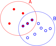
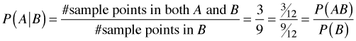
Fig. 1 The sample space S with events
A and B (R code)
Bayesian inference is as old as statistics itself. The frequentist approach on the other hand is a more recent innovation and derives from the uncomfortable marriage of methodologies developed by the Neyman-Pearson-Wald school (hypothesis testing) and the Fisherian school (everything else). While there are fundamental differences in the Bayesian and frequentist approaches that are difficult to reconcile, most statisticians treat them as just two options on a menu and are willing to use the tools they offer without necessarily embracing the accompanying baggage.
The history of Bayesian statistics began in 1763 with a paper written by Thomas Bayes in which he outlined a formula that has come to be called Bayes rule. In the early 1900s the frequentists (Fisher, Neyman, and Pearson) rejected the Bayesian approach, after which it temporarily slipped into obscurity and all focus shifted to frequentist methods. Bayesian methods experienced a revival in the early 1990s so much so that Bayesian approaches are now the hottest area of modern statistics.
While there has been considerable rancor in the literature (particularly among scientists) with regard to these two approaches, I think it is fair to say that Bayesian inference has always been recognized as being the more legitimate approach to doing statistics. Because Bayesian inference was difficult to carry out except in a few fairly artificial cases, the frequentist approach has held sway by default. Except for a few universities that have built their reputation on being Bayesian hotbeds, (Duke, for example), most statistics departments have tended to include only token representatives of the Bayesian viewpoint among their faculty.
This situation dramatically changed about 20 years ago. Using methodologies originally developed by physicists, Bayesian inference is now easy to do. Furthermore Bayesian methods are able to solve problems that are currently impossible for the frequentist approach to solve. This has generated a great deal of interest in Bayesian statistics among scientists in general. I introduce Bayesian statistics here not as an alternative to frequentist statistics but as a collection of tools that can be useful in many instances.
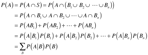
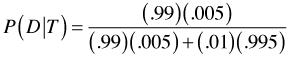
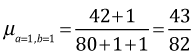
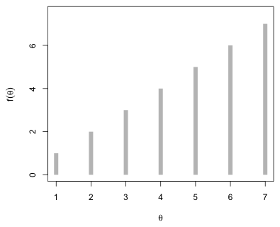
On first pass, Bayes rule would seem to be just a trivial extension of the concept of conditional probability. I begin by reviewing the definition of conditional probability. Let Fig. 1 represent a sample space S consisting of 12 equally likely sample points. The events A and B are the subsets of sample points shown in the figure. Under the equally likely assumption we have the following.
Fig. 1 The sample space S with events
A and B (R code)
Conditional probabilities effectively change the sample space. For instance, P(A|B) restricts the sample space to B and is calculated under the equally likely scenario by counting up the number of sample points that are both in A and B and dividing by the number of sample points in B. Formally we have
With this background, Bayes rule can be derived as follows. Let A and B be any two events. Using the definition of conditional probability we can write the following.
Having solved for the joint probability ![]() in each expression we can set the results equal to each other.
in each expression we can set the results equal to each other.
This latter formula is essentially Bayes rule but not as it is usually written. Imagine a set of events ![]() that are pairwise disjoint and partition the sample space S such that
that are pairwise disjoint and partition the sample space S such that ![]() , then we can write P(A), the denominator in the above expression, as follows.
, then we can write P(A), the denominator in the above expression, as follows.
Substituting this expression for P(A) in the denominator of the formula for P(B|A) given above yields Bayes rule.
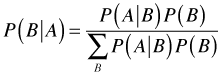
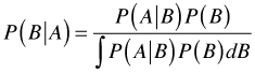
If B is continuous, the sum is replaced by an integral.
The following Bayes rule problem is typical of the kind that appears in textbooks on elementary probability theory and biostatistics.
Suppose a certain drug test is 99% sensitive and 99% specific, that is, the test will correctly identify a drug user as testing positive 99% of the time, and will correctly identify a non-user as testing negative 99% of the time. This would seem to be a relatively accurate test, but Bayes' theorem can be used to demonstrate the relatively high probability of misclassifying non-users as users. Let's assume a corporation decides to test its employees for drug use, and that only 0.5% of the employees actually use the drug. What is the probability that, given a positive drug test, an employee is actually a drug user?
The assertions made in the problem can be formulated as conditional probabilities. Let's make the following identifications.
D = event that an employee uses drugs
Dc = event that an employee does not use drugs
Notice that these two events form an exhaustive partition of our sample space, i.e., ![]() . Either an employee uses drugs or he/she does not. Continuing with our identifications, let
. Either an employee uses drugs or he/she does not. Continuing with our identifications, let
T = event that an employee tests positive on a drug test
Tc = event that an employee tests negative on a drug test
These two events form a second partition of our sample space, i.e., ![]() . Sensitivity and specificity are formulated as conditional probabilities.
. Sensitivity and specificity are formulated as conditional probabilities.
sensitivity:
specificity:
Conditional probabilities satisfy the laws of probability so given drug use either an individual tests positive or not. Thus we also know
![]() and similarly
and similarly ![]() . We're also told
. We're also told ![]() , from which it follows
, from which it follows ![]() because these two probabilities have to add to 1. We're asked to find
because these two probabilities have to add to 1. We're asked to find ![]() . From the definition of conditional probability we have
. From the definition of conditional probability we have
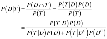
where in the last step I use Bayes rule in which our sample space of people with positive tests is partitioned as ![]() . Plugging in the numbers we obtain the following.
. Plugging in the numbers we obtain the following.
This low accuracy seems anomalous given the apparently high precision of the tests until we realize that the activity being tested for is quite rare. While I present this largely as an illustration of Bayes rule in action there is another message to take home from this example. The order of the events in the conditional probability truly matters. In the example ![]() and
and ![]() are not only different conceptually but also very different numerically.
are not only different conceptually but also very different numerically.
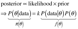
In the Bayesian approach to statistics Bayes rule becomes both a method of estimation and a way to make inferences. Here's Bayes rule again in its continuous form.
Now let B = θ, a parameter, and A = data, then Bayes rule can be written as follows.
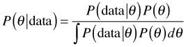
With these definitions we can express Bayes rule as
![]()
where the constant of proportionality is give by the reciprocal of the integral shown above. Thus with Bayes rule we update the prior probability of θ via the likelihood to obtain the posterior probability of θ.
The posterior probability is a statement of our belief about the state of nature. It takes into consideration our prior beliefs as well as what we've learned from our data. If we have no substantive prior beliefs then we can use what are called "vague" or "uninformative" priors. In these cases we essentially derive all of our inference from the likelihood, just like in the frequentist approach to statistics. A subtle difference is that because we used Bayes rule to set up our problem the conclusions we draw about the parameters can be formulated as probability statements.
To illustrate the differences between the frequentist and Bayesian approaches to parameter estimation, I apply the two methodologies to a common problem. The problem is simple enough that classical Bayesian methods can be used. An experiment is carried out to determine the seed germination success of a particular genetic strain. Eighty seeds were sewn separately in a single tray placed in a greenhouse. The total number of seeds that successfully germinated was recorded. Suppose we observe that 42 seeds germinated. We make the assumptions that the seed are independent, so that the individual seeds in a given tray do not interfere with each other, and that the seeds have an identical germination success rate p.
Regardless of whether we are taking a frequentist or Bayesian approach, we begin by writing down the likelihood for this experiment, the probability of observing the data that we observed. Let Xi = outcome for seed i. This outcome is 1 if the seed germinated, and 0 otherwise. If we list the outcome for each seed in order, then the probability of our data is the following.
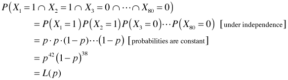
This is an example of what's called a product Bernoulli distribution, which is closely related to the more familiar binomial distribution.
Frequentists work exclusively with the log-likelihood.
![]()
To find the maximum likelihood estimate of p using calculus we can differentiate the log-likelihood, set the result equal to zero, and solve for p. For this problem these steps are easy.
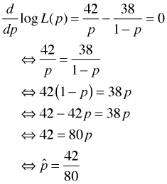
Observe that the estimate is just the total number of successes (germinations) divided by the total number of trials, i.e., the fraction of successes. As is often the case the maximum likelihood estimate is a fairly natural estimate. To obtain this result numerically we can write a function that calculates the negative log-likelihood as a function of p and then use the nlm function to find its minimum.
This is the total number of successes divided by the total number of trials.
Using the Hessian we can calculate a 95% Wald confidence interval for the proportion.
Bayesians also begin with the likelihood.
![]()
In addition to the likelihood a Bayesian requires a prior probability for p. The prior probability is a probability distribution that summarizes our knowledge about p before we collected the current data. In a classical Bayesian analysis we would like a probability distribution for the prior that readily combines with the likelihood so that the posterior distribution can be obtained by inspection. Furthermore a prior for p should be a probability model that assigns non-zero probabilities to values in the interval (0, 1) and zero values outside this interval. The beta distribution is an example of such a probability distribution. The probability density function of a beta distribution with parameters a and b is the following.
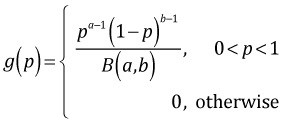
where B(a, b) is a normalizing constant called the beta function. The mean of a beta distribution in terms of its parameters is . Using a generic beta prior for p, the posterior probability of p can be written as follows.
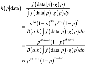
If we ignore the normalizing constants in the denominator, we see that the numerator has the form of a beta distribution with parameters 42 + a and 38 + b. Thus it must be the case that the normalizing constant must reduce to B(42 + a, 38 + b) and hence the posterior distribution is also a beta distribution.
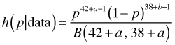
The mean of this distribution is
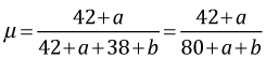
In order to agree with the frequentist estimate, we need to choose an uninformative prior for p. For a proportion bounded on the interval [0, 1] a natural choice is the uniform distribution on this interval. A uniform distribution on (0, 1) has the constant density f(p) = 1 and is a special case of a beta distribution in which a = b = 1. For a Bayesian point estimate of p we can use the mean of the posterior distribution that is given by
 = 0.5243902
Notice that the Bayesian estimate of p is similar but not identical to the frequentist estimate. The difference between the two estimates would be smaller with a larger sample size because the influence of the prior would be further reduced.
The beta distribution is referred to as a conjugate distribution of the product Bernoulli distribution (more generally, it is a conjugate distribution of the binomial distribution). They are conjugates because the product of the two distributions yields a new distribution that is of the same form, in this case a beta distribution. Historically this was how Bayesian estimation proceeded. We construct a likelihood and then try to find a suitable prior such that the prior is a conjugate to the likelihood, or is such that the normalizing integral in the denominator of Bayes rule that results can be evaluated. The problem with the classical approach is that it restricts the use of Bayesian methods to only very simple problems. When we turn to regression problems in which there are multiple parameters of interest each with their own priors there is no simple way to select the priors so that the corresponding posterior distribution can be determined.
The manner in which statisticians carry out Bayesian estimation changed dramatically in the early 1990s. Today Bayesian analysis is carried out using a set of techniques referred to as Markov Chain Monte Carlo methods that make it possible to sample from the posterior distribution, for a given prior and likelihood, without the need to obtain an explicit formula. Markov chain Monte Carlo (MCMC for short) has two components to its name: Monte Carlo and Markov chain.
So a Markov chain is how we get to the posterior distribution and Monte Carlo is how we obtain samples of that posterior distribution once we get there. Markov chain Monte Carlo doesn't return a formula for the posterior distribution, just a set of values. But with a large enough sample we can characterize most features of interest about the posterior distribution—quantiles, means, medians, etc. The trick in Markov chain Monte Carlo is to find a Markov chain whose stationary distribution is ![]() . With such a Markov chain we just let it run for a while (the so-called burn-in period) to give the chain time to reach its stationary distribution. Once there the chain will roughly visit values in the stationary distribution in proportion to their probabilities. Thus values in more probable regions of the distribution will be visited more often than values in the tail of the distribution.
. With such a Markov chain we just let it run for a while (the so-called burn-in period) to give the chain time to reach its stationary distribution. Once there the chain will roughly visit values in the stationary distribution in proportion to their probabilities. Thus values in more probable regions of the distribution will be visited more often than values in the tail of the distribution.
A full discussion of MCMC methods and why MCMC works is beyond the scope of this course. Some of the references cited at the end of this document provide more information. The programs BUGS and JAGS are adaptive in their choice of method. They will use Gibbs sampling, adaptive rejection sampling, the Metropolis algorithm, or various other MCMC methodologies depending on the nature of the problem you submit. To give a hint at the flavor of what's involved I briefly describe the logic behind two of these MCMC methods: the Metropolis algorithm and Gibbs sampling.
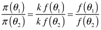
The Metropolis algorithm originates from work in statistical physics dating back to the 1950s and was adapted for Bayesian estimation only in the last 25 years. The method uses the fact that knowing the full formula for the posterior distribution, including the normalizing constant, is unnecessary if one only needs to deal with the ratios of posteriors. Ignoring the details of the normalizing constant Bayes rule can be written as follows.
where k is the normalizing constant. So, when we look at the ratios of the posterior densities at two distinct values of the parameter, θ1 and θ2, the normalizing constant cancels. So, we only need to work with the likelihood and the prior, the two quantities for which we have formulas.
The Metropolis algorithm uses what's called a proposal distribution (also a jumping or instrumental distribution) to generate candidate values of θ. The proposal distribution is denoted
![]()
In the Metropolis algorithm the proposal distribution must be one that is symmetric, i.e., ![]() . In another variation, the Metropolis-Hastings algorithm, the symmetry requirement is replaced with a more general condition.
. In another variation, the Metropolis-Hastings algorithm, the symmetry requirement is replaced with a more general condition.
At step t – 1 of the Metropolis algorithm, a new candidate value ![]() is drawn from the proposal distribution. A form of rejection sampling is then used to decide if we should keep this new value. We calculate
is drawn from the proposal distribution. A form of rejection sampling is then used to decide if we should keep this new value. We calculate
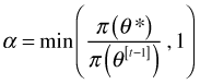
and the new parameter value ![]() is accepted with probability α. In the Metropolis-Hastings algorithm the formula that is used for α is slightly more complicated in that it also involves a ratio of the proposal distributions. In practice if α < 1 then we draw a random value u from the uniform distribution on (0, 1) and keep
is accepted with probability α. In the Metropolis-Hastings algorithm the formula that is used for α is slightly more complicated in that it also involves a ratio of the proposal distributions. In practice if α < 1 then we draw a random value u from the uniform distribution on (0, 1) and keep ![]() if u ≥ α.
if u ≥ α.
It turns out that the series of θ values generated by this algorithm forms a Markov chain whose stationary distribution is the desired posterior distribution ![]() . The Markov chain generated by the Metropolis-Hastings algorithm converges to
. The Markov chain generated by the Metropolis-Hastings algorithm converges to ![]() regardless of the choice of proposal distribution q, but the choice of q can affect how fast the convergence takes place.
regardless of the choice of proposal distribution q, but the choice of q can affect how fast the convergence takes place.
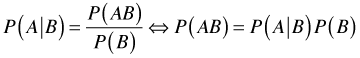
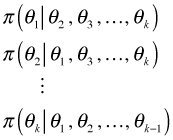
Here's a trivial illustration of how the Metropolis algorithm might work in practice. Suppose there are only seven possible values of θ, the numbers 1 through 7, and that we can evaluate the prior, the likelihood, and their product at each of these seven values. The product of the prior and the likelihood is the numerator of Bayes rule and is referred to as the target distribution, ![]() . It's the posterior density without the appropriate normalizing constant. For our example with seven distinct values of θ, suppose the target distribution takes the following form, where for convenience I've chosen f(θ) = θ (Fig. 2).
. It's the posterior density without the appropriate normalizing constant. For our example with seven distinct values of θ, suppose the target distribution takes the following form, where for convenience I've chosen f(θ) = θ (Fig. 2).
 |
| Fig. 2 Hypothetical target distribution. |
We begin by choosing one of the seven possible values of θ at random. This is our starting value. Next we need a proposal distribution, a way of generating new values of θ given the current value of θ. A simple choice is to either select the observation immediately to the left of θ with probability 1/2 or to select the observation immediately to the right of θ with probability 1/2. Thus if the current value of θ is θi, we next choose either θi – 1 or θi + 1 with equal probabilities. (Note: we would need to treat the endpoints θ = 1 and θ = 7 as special cases.) We can implement this by choosing a random number between 0 and 1. If the random number is less than 0.5, we choose θi – 1; if this number is greater than 0.5 we choose θi + 1.
Having selected a candidate value we have to decide whether to keep it (move there). For that we evaluate the target distribution function at the candidate value and compare it to the value of the target distribution function at the current value. If the target distribution is larger at the candidate value, so that the ratio of the target distributions is greater than 1, we move there. If the ratio is less than one then we move to the candidate value with probability equal to the ratio. For the target distribution in Fig. 2 our decision rule is the following.
 , otherwise we stay where we are.
This leads to the formal decision rule given previously. To see how this would work in practice suppose the random starting point is θ = 4. I generate six random numbers between 0 and 1.
So after five steps our Markov chain consists of the values {4, 5, 4, 5, 4}. The claim is that if we carry out this protocol long enough the relative frequencies of the elements of our sample will correspond to the probabilities of the posterior distribution (which is a multiple of the target distribution). The rationale for this assertion is that our choices in moving from one point to another are entirely determined by the relative magnitudes of the posterior probabilities.
For the case in which there is a continuum of possible values for θ we need a more elaborate proposal distribution. A typical choice might be a normal distribution centered at the current value with a standard deviation that is treated as a tuning parameter. Because it generally takes a while to explore the parameter space, particularly if we start in an unrepresentative portion of it, the Metropolis algorithm requires a burn-in period. The observations obtained during the burn-in period are discarded. Because also it will take a while for the relative frequencies in our sample to stabilize around those of the posterior distribution, the Metropolis algorithm needs to be run for a long time after the initial burn-in period. (There are a number of diagnostics that have been developed for determining how long to run the algorithm and when to terminate the burn-in period.) Once we're satisfied that we're sampling from the stationary (posterior) distribution, we let the Markov chain run some more this time saving the values it generates. The values we obtain are then used to obtain Monte Carlo estimates of whatever characteristics of the posterior distribution we desire.
The Gibbs sampler is another of the Markov chain Monte Carlo methods implemented in the software BUGS and JAGS. The Gibbs sampler yields a Markov chain whose stationary distribution is the posterior distribution we want. Thus after a finite amount of time we're guaranteed that the sequential values of the Markov chain are correlated samples from the desired posterior distribution. The relative frequency of observations from different intervals corresponds approximately to the probabilities defined by the posterior distribution over those intervals.
Suppose ![]() depends on k parameters
depends on k parameters ![]() . Then the Gibbs sampler requires k conditional probability statements of the form
. Then the Gibbs sampler requires k conditional probability statements of the form
These probabilities are often obtainable from hierarchical models when the models are formulated from a Bayesian perspective. Typically the basic regression model is itself a conditional statement, the random effects are conditional on the values of parameters of a normal distribution, and all the remaining parameters are conditional on their priors.
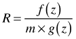
With the conditional probabilities formulated we choose starting values ![]() and then use the probability statements one by one to update these values by drawing new values from the full conditional probability distributions. At stage j of the iteration the update equations will look as follows.
and then use the probability statements one by one to update these values by drawing new values from the full conditional probability distributions. At stage j of the iteration the update equations will look as follows.
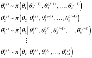
Notice that once a new value is generated it is immediately used as the conditioning value for the remaining parameters in all subsequent conditional probability distributions at stage j. This is clearly a Markov chain. It also turns out to be an ergodic Markov chain.
![]() ,
,
i.e., in the limit the probability of going from ![]() to
to ![]() in n steps depends only on the final state. When the Gibbs sampler is formulated from the likelihood and priors of a Bayesian model, the limiting probability
in n steps depends only on the final state. When the Gibbs sampler is formulated from the likelihood and priors of a Bayesian model, the limiting probability ![]() is in fact the desired posterior probability.
is in fact the desired posterior probability.
So, we set up the Gibbs sampler and we let it run for a while (the burn-in period) to give the chain time to "reach" its limiting distribution. Once there the chain visits values roughly in proportion to their probabilities. With a large enough sample of chain values we can obtain estimates of these probabilities and use them to estimate other parameters of interest. Bayesian problems are well-suited for the Gibbs sampler because they are already based on a series of conditional probability statements. The good news is that we don’t have to set up the equations for the Gibbs sampler ourselves, WinBUGS and JAGS do it for us based on the model definition file we give it.
When conjugate priors are chosen so that the posterior distribution has a known form WinBUGS can bypass all this and sample directly from the posterior distribution using standard algorithms. One such standard algorithm is the inversion method. When this is not the case WinBUGS can use a method called adaptive rejection sampling. Rejection sampling requires that we can find an envelope function, g(x), that when multiplied by some constant, m, is greater than the true posterior density, f(x), at all values of x. The envelope function needs to be one from which sampling is easy. Having drawn a value z from the envelope function, we examine the ratio R,
We then draw a number u from the uniform distribution on the interval (0, 1). If R > u, we accept the value of z as the new value of our parameter. Otherwise we keep the old value. The envelope function used by BUGS is constructed from a set of tangents to the log of the conditional density.
For the frequentist everything hinges on the notion of repeated sampling. In the informal definition of probability the probability of an event represents the long range relative frequency of the occurrence of that event. To say that the probability of heads is one half when a fair coin is tossed once means that if we were to flip a fair coin repeatedly the long run relative frequency of heads is one half. (Note: another way to interpret probability in this example is to treat the possible outcomes of a coin flip as equally likely.)
Statistical inference derives from the sampling distribution of a statistic. The sampling distribution is the set of estimates obtained when all possible samples are selected from a target population. Properties of a statistic (unbiasedness), standard errors, etc. derive from the sampling distribution of that statistic.
Implicit in the frequentist approach to estimation is that there is a fixed quantity in nature, the parameter θ, that we wish to measure with a statistic. For example, the bias of a statistic is the difference between mean of the sampling distribution of the statistic and the true value that is being estimated. So, for a frequentist it is parameters that are fixed while it is the data that are random. This is diametrically opposed to the Bayesian point of view. For a Bayesian it is the data that are fixed and parameters that are random.
The notion that the parameter is a fixed quantity in nature causes problems in interpretation for the frequentist. When we construct a confidence interval for a parameter we like to treat the interval as a probability statement for the parameter—the set of likely values it might take. But in truth if the parameter is fixed then it is either in the interval we've constructed or it's not. There's no probability associated with it. The probability instead derives from the sampling distribution. We call it a 95% confidence interval because we're guaranteed that 95% of the intervals we might have constructed, if we had obtained all possible samples from the population, do in fact contain the true parameter value. All we can do is hope that this is one of the lucky ones.
It's been said that constructing a 95% confidence interval is analogous to running from an elephant while shooting an elephant gun over your shoulder. Did you hit it? You don't know but you know that 95% of the time an elephant gun is known to stop an elephant. You just hope this is one of those times. The bottom line is that when θ is treated as real and fixed, then it's only our methods that can have probability associated with them.
The frequentist perspective uses p-values as measures of evidence against hypotheses, but the p-value is a measure of how likely are the observed data under the null hypothesis, i.e., ![]() . This doesn't address the probability of the null hypothesis, for that we need
. This doesn't address the probability of the null hypothesis, for that we need ![]() . So the p-value addresses the wrong probability. We've seen from our simple drug example application of Bayes rule that the order matters in conditional probability statements. Practically speaking the frequentist is trying to trying to draw inference about whether a specific individual who tested positive on a test is a drug user using only the sensitivity of the test.
. So the p-value addresses the wrong probability. We've seen from our simple drug example application of Bayes rule that the order matters in conditional probability statements. Practically speaking the frequentist is trying to trying to draw inference about whether a specific individual who tested positive on a test is a drug user using only the sensitivity of the test.
A Bayesian has other problems with p-values beyond the fact that they estimate the wrong probability. By definition a p-value is the probability under the null hypothesis of obtaining data as extreme or more extreme than the data one actually obtained. A Bayesian would wonder why we are basing our decision about the null hypothesis using data we didn't obtain. Shouldn't we base our decisions on the evidence at hand and not on the evidence we might have obtained?
In the Bayesian approach, probability is a matter of opinion. It still must follow the standard rules of probability (the Kolmogorov axioms, for instance), but other than that things are pretty flexible. For this reason Bayesians are said to take a subjective approach to probability (as opposed to the "objective" approach of the frequentists).
As far as the existence of a true value of θ in nature, Bayesians are of an open mind. θ may or may not be real, but in the Bayesian perspective it doesn't matter. All we know about θ is what we believe about it. As knowledge accumulates our beliefs about θ become more focused. Since the value of θ is a matter of belief, and probability is a matter of belief, for all intents and purposes θ can be viewed as a random quantity. Consequently to a Bayesian parameters are random variables, not fixed constants. As a result confidence intervals pose no philosophical dilemma for a Bayesian. Since parameters are random we can make probability statements about their values. Thus a confidence interval for θ is a probability statement about the likely values of θ. To avoid confusion with frequentist confidence intervals, Bayesians often call their intervals "credible intervals".
A Bayesian takes pride in the fact that Bayes rule as formulated above essentially encapsulates inductive science in a single formula. In science we develop theories about nature. Observation and experiment then cause us to modify those theories. Further data collection causes further modification. Thus science is a constant dynamic between prior and posterior probabilities, with prior probabilities becoming modified into posterior probabilities through experimentation at which point they become the prior probabilities of future experiments. Thus the Bayesian perspective accounts for the cumulative nature of science.
The frequentist retort is that this is a mischaracterization of science. Science is inherently objective and has no use for subjective quantities such as prior probabilities. Science should be based on data alone and not the prejudices of the researcher.
The Bayesian rejoinder to this is first that science does have a subjective component. The "opinions" of scientists dictate the kinds of research questions they pursue. In any case if there is concern that a prior probability unfairly skews the results, the analysis can be rerun with other priors. In Bayesian analysis it is fairly typical to carry out analyses with a range of priors to demonstrate that results are robust to the choice of prior.
In fact both schools of thought are correct here. While Bayesians may have described the ideal scientific method, in truth consensus in science is informal at best. Perhaps there should be a current prior probability in vogue for everything in science, but typically there isn't. Without this consensus the inherent subjectivity of priors does seem to be a problem.
It's interesting then that Bayesians and frequentists reject the other's approaches for essentially the same reason.
Until Markov chain Monte Carlo came along this entire argument was moot because very few interesting problems could be solved using Bayes rule. The reason lies in the integral that appears in the denominator. For most higher dimensional scenarios evaluating this integral is an intractable problem.
Historically the only estimation problems Bayesians were able to solve were trivial ones where the integral can be ignored because the form of the posterior probability can be determined by inspection. These situations involve what are called conjugate priors in which the likelihood and prior combine in a nice fashion so that the posterior probability can be determined without integration. For instance, a normal prior and a normal likelihood yield a normal posterior of a known form. A binomial likelihood coupled with a beta prior yield a beta posterior of known form. There are a number of other examples of conjugates, but the list is not very long. Now that MCMC methods have obviated this problem by sampling from the posterior distribution directly the pendulum of opinion has swung back in the Bayesian direction.
While there are many good reasons for taking a Bayesian perspective, I address this section to someone who is committed to doing statistics from a frequentist perspective. So why in general should a frequentist care about the Bayesian approach and have to grapple with the issue of choosing prior probabilities? I give two reasons.
The upstart of this is that MCMC can be used to obtain parameter estimates for distributions when it is far too complicated to obtain these estimates using ordinary frequentist optimization methods. The typical situations where the Bayesian perspective may be necessary are the following:
One or more of these four conditions is typical in ecology. The only real problem from a practical standpoint with using Markov chain Monte Carlo in model estimation is that it exacerbates the temptation to toss parsimony out the window and to fit extremely complicated models. This temptation should be resisted at all costs!
Software such as WinBUGS and JAGS that implement Markov chain Monte Carlo (MCMC) methodology can be to carry out Bayesian estimation. BUGS is an acronym for "Bayesian inference Using Gibbs Sampling" while JAGS is an acronym for "Just Another Gibbs Sampler". Both use the BUGS programming language to formulate the likelihood of our data under our chosen model along with prior distributions for the model parameters. Based on the information we provide it, WinBUGS and JAGS set up the appropriate Gibbs sampler (or some alternative MCMC method) that yields Markov chains that we can then track.
To illustrate the use of this software I refit the analysis of covariance model we considered in lecture 9. The data were taken from Crawley (2002) who described three variables of interest.
Our final model from lecture 9 was the following.
We will fit this same model using Bayesian methods and compare the estimates to those returned by lm.

Fig. 3 R file menu choices
WinBUGS is a stand-alone package that is not particularly easy to use. Andrew Gelman of Columbia University has written an R package, arm, that among other things permits running WinBUGS models from within R by calling on the bugs function from the R2WinBUGS package. This simplifies the use of WinBUGS considerably because we can use R to set up the analysis and process the results and then use WinBUGS only to fit the model.
JAGS also uses the BUGS programming language with some minor differences. It is not stand-alone software but requires R in order to run. The R2jags package can be used to run JAGS models from R. The jags function from this package returns output that matches the format of the output generated by WinBUGS.
To run WinBUGS using bugs requires the following.
WinBUGS can be installed to any location on your machine. If WinBUGS is not installed in the default location, C:\Program Files\WinBUGS14, then the correct path needs to be specified when you invoke WinBUGS from within R. To run JAGS you need the JAGS software and the R2jags package from the CRAN site.
At the core of every WinBUGS or JAGS run is a model definition file that specifies the details of the model. This is a text file written in the BUGS language. It should be created in Notepad or some other text editor. It is important that the working directory of R be set to the directory where this text file has been saved. The working directory can be set by making a menu choice or by using the setwd command at the R console. To set the working directory using menus on Windows go to the File menu and select Change dir... (Fig. 4). In the dialog box that appears set the directory to match the location where the WinBUGS model definition file lives. This directory now becomes the default location where R will save graphics and other output. On a Mac choose R > Preferences > Start up and make the changes in the Initial Working Directory section. I prefer to use the setwd command from the console (see below).
IMPORTANT CAVEAT!! Do not bury your BUGS program inside many folders. Try to store it only a few layers deep. More importantly, do not save it in folders with long and complicated names. WinBUGS will fail to run and give you a completely incomprehensible error message to boot.
WinBUGS likes things simple. For instance WinBUGS accepts only numeric data. Character data and factors are not allowed so factors need to be converted to a set of dummy variables. In addition variables must be entered into WinBUGS in a special way. To facilitate this I begin by pulling out the individual variables of the data frame ipo that we will need for the regression analysis. In doing so I try to keep the variable names simple and generic.
The BUGS model definition file that we'll construct at one point makes use of the number of observations in the data set as a constant. So I calculate this value in R and assign the result to another object.
Next I write the Bayesian model using the BUGS language. Much of the language resembles R but with subtle differences. The language is documented in manuals available at the site where you downloaded WinBUGS and/or JAGS. I enter the lines in NotePad and save the resulting file as ipomodel.txt. Here's the model definition file followed by a line-by-line explanation.
BUGS code looks just like R code but with important differences. BUGS code is used to specify the model. The lines of code are not instructions that are executed. In fact BUGS code is not executed at all; it is a declarative language. Although lines are entered sequentially, they’re not interpreted sequentially. BUGS parses the entire model and then runs a process. BUGS can make use of for loops for model specification but there use is just a matter of convenience. There are six kinds of BUGS objects.
BUGS uses probability function with names that match many of R's probability functions but there is a twist. For instance the dnorm function is parameterized in terms of precision (reciprocal variance) rather than the standard deviation. Secondly, dnorm is not really a function in WinBUGS(as it is in R) but is just a label for the normal distribution. The ~ as used here has the meaning it has mathematically, namely "is distributed as", and is not the formula operator of R.
In this course we will use the following strategies for setting uninformative priors for model parameters.
The most important modeling strategy when using BUGS is to start simple and complexify gradually each time checking that the current model works and makes sense before moving to a more complex model.
With the model saved to the working directory, we enter the following three lines back at the console prompt in R.
These three lines create objects that will be passed to WinBUGS/JAGS for use in estimating the model.
I next set the working directory (if this hasn't already been done using the menu, Fig. 3) using the setwd function. The working directory is the one that contains the BUGS model definition file. It is not a good idea to bury things in folders that are many layers deep. The containing folders should also have fairly simple names. If you violate either of these recommendations, WinBUGS may fail to run (and the error message you get will be completely cryptic). To see what the current working directory is use the getwd() command.
We're now ready to run the model. On a Mac I load the R2jags package (which must be initially downloaded from the CRAN site because it's not part of the standard R installation--be sure to check the install dependencies box when you download it) and make the following call using the jags function from R2jags.
On Windows I load the arm package (which must be initially downloaded from the CRAN site because it is not part of the standard R installation) and make the following call using the bugs function from arm.
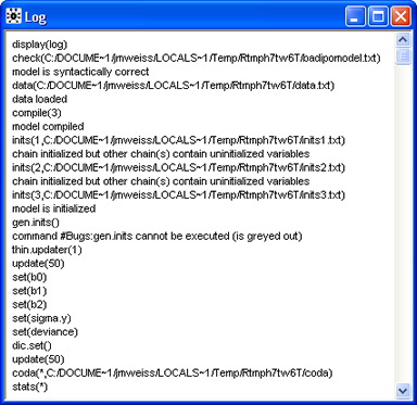
Fig. 4 WinBUGS report on the model
Shown below is an explanation of each of the arguments of jags and bugs.
JAGS provides minimal output. WinBUGS provides a lot more information. Fig. 4 shows the partial contents of the log window in WinBUGS from this run. The important thing to observe is that there are no error messages here.
The rest of the log (Fig. 5) displays summary statistics and graphs of individual Markov chains for different parameters and statistics. With only 100 iterations contributing to these reports, there is little to be learned from them. Observe though that the last 50 iterations of the chains already appear to be mixing.
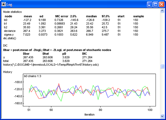
Fig. 5 Additional information in the WinBUGS log window
Since there were no errors we can now run the model for real with a reasonable number of iterations. In the run below I specify 10,000 iterations. By default the bugs function is set up to treat the first half of the iterates as part of the the burn-in period. So the first 5,000 iterations of this run are discarded and only the values from the second half of the run are saved. (This can be changed by specifying a value for the n.burnin argument of bugs.)
Furthermore the bugs function uses a default thinning rate of max(1, floor(n.chains*(n.iter-n.burnin)/1000). The n.thin argument can be used to override this default. With three chains, n.iter = 10000, and n.burnin = 5000, the thinning rate is 15. Thus only every 15th simulation value is saved. With 3 chains this means BUGS will return 1002 (3 times 334) samples, which, if convergence has been attained, will be samples from the posterior distributions of each parameter. It is not necessary to keep the debugger on at this point, but I do so in order to inspect some of trace plots of the Markov chains that are produced. JAGS thins things so that 1000 observations remain in each chain. Thus JAGS returns three times as many observations as does WinBUGS.
Fig. 6 shows plots of the three Markov chains for the standard deviation parameter, sigma.y. Observe that trajectories are thoroughly interdigitating indicating that the chains have mixed fairly well. The fact that all three chains are traversing the same range of y-values provides evidence that the chains are now sampling from the posterior distribution of sigma.y. The fact that the individual chains are jumping around a lot indicates there is very little autocorrelation in the chains. This is good because it implies that the returned observations are nearly independent meaning that our effective sample size is close to the actual sample size.
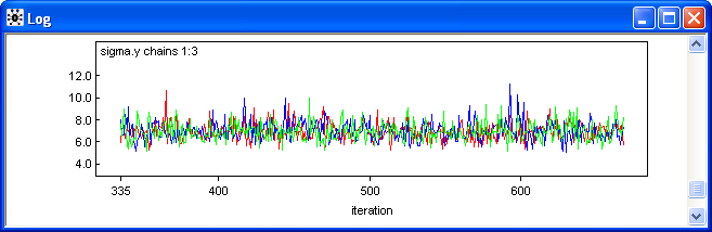
Fig. 6 Trace plots of the individual Markov chains for the standard deviation of the response
This last model would be fit using JAGS as follows.
To unfreeze the R console, close the WinBUGS window. We can view summary statistics for the posterior distributions of each parameter by typing the name of the object to which the bugs output was assigned.
For each parameter, n.eff is a crude measure of effective sample size,
and Rhat is the potential scale reduction factor (at convergence, Rhat=1).
DIC info (using the rule, pD = Dbar-Dhat)
pD = 4.0 and DIC = 271.6
DIC is an estimate of expected predictive error (lower deviance is better).
The output shows the mean, standard deviation, and various quantiles of the posterior distributions of the four parameters b0, b1, b2, and sigma.y. To be sure that we are actually sampling from the posterior distribution we should examine the column labeled Rhat. Rhat is the mixing index. Numerically it is the square root of the variance of the mixture of all the chains divided by the average within-chain variance. If the chains are mixed these values should be roughly the same yielding a ratio of approximately 1. Since Rhat is reported to be 1 for all the parameters this is evidence that the chains are well-mixed and that the Gibbs sampler is sampling from the posterior distribution.
A lot of other useful information is contained in different components of the object created by the bugs function.
With JAGS this same information is contained in the $BUGSoutput component of the jags object.
So with the jags object we access the these components as ipo.1j$BUGSoutput$sims.matrix, ipo.1j$BUGSoutput$summary, etc.
The sims.array component arranges the information in a three dimensional array, a set of matrices, one for each parameter. The individual matrices contain the samples obtained from each Markov chain as separate columns listed in the order the sampled observations were obtained. Thus each column records the sampling history for that Markov chain. For the current example each parameter is represented by a 334 × 3 matrix. Below I display the first two sampled observations in each chain for all of the parameters.
[,1] [,2] [,3]
[1,] -135.1 -136.3 -132.1
[2,] -112.3 -138.2 -133.8
, , b1
[,1] [,2] [,3]
[1,] 24.24 24.77 23.84
[2,] 21.73 24.49 24.16
, , b2
[,1] [,2] [,3]
[1,] 38.22 35.02 37.19
[2,] 30.64 42.11 37.07
, , sigma.y
[,1] [,2] [,3]
[1,] 5.911 7.994 7.598
[2,] 7.157 6.489 6.518
, , deviance
[,1] [,2] [,3]
[1,] 266.4 269.3 267.1
[2,] 266.5 267.9 264.7
We can use the information contained in the sims.array component to make our own trace plot of the Markov chains in order to evaluate mixing.
In the sims.list component, the chains are combined into a single long vector and their order is randomly permuted (so that the actual sample history of the observations is lost). The individual parameters can be accessed as list objects, as in ipo.1$sims.list$b0, ipo.1$sims.list$b1, etc. Below I select the first five elements of each parameter and in the second call I request the first five samples from the posterior distribution of the parameter b0.
In the sims.matrix component the three chains are combined again but this time the samples from the posterior distributions occupy the columns of a matrix. As was the case with the sims.list component, the row order of the observations in the sims.matrix component has been randomly permuted (so that the actual sample history is lost).
We can use this information to calculate our own summary statistics. Here are the means of the sampled posterior distributions. The values match what's reported in the summary table above.
It's useful at this point to contrast the estimates obtained from the Bayesian posterior distributions with what we obtained previously from fitting the model using the lm function and ordinary least squares.
The ordinary least squares results for this model are the following.
In general we don't expect the frequentist and Bayesian estimates to be the same, but for well-defined, trivial problems such as this with truly uninformative priors, we expect them to be close. If the differences in the estimates are large there are three possible explanations.
Explanation (1) can be ruled out by looking at chain diagnostics, as we've done. Explanation (3) is always a possibility. What's uninformative for one problem may be informative for another. The intercept in this model is an order of magnitude larger than either of the effect estimates. Suppose I increase the precision of all the priors by a factor of 100 in the model definition file. I save the new file as badipomodel.txt. The changes to the old model definition file are indicated in red.
I rerun the model with the new model definition file and then display the summary statistics of the posterior distributions again.
For each parameter, n.eff is a crude measure of effective sample size,
and Rhat is the potential scale reduction factor (at convergence, Rhat=1).
DIC info (using the rule, pD = Dbar-Dhat)
pD = 3.8 and DIC = 271.2
DIC is an estimate of expected predictive error (lower deviance is better).
Now the Bayesian and frequentist estimates of the intercept are much further apart. So what went wrong? Choosing a precision of .0001 is equivalent to a normal variance of 10000, or a normal standard deviation of 100. This says that we are 95% certain for instance that the estimate of the intercept lies in the interval (–200, 200). The estimate of the intercept turns out to be –126, so clearly the prior we're using is quite informative. Here the standard deviation is the same order of magnitude as the parameter we're trying to estimate. To be an uninformative prior we need the standard deviation to be at least a couple of orders of magnitude greater than the estimate, yielding a range of uncertainty that is wider than the range of reasonable values of the parameter.
The obvious solution would be to always choose the precision to be very small. The problem with this is that in complicated problems this can lead to numerical instability. BUGS can become computationally unstable when the priors on parameter values are given too wide a range. For instance if I change the prior for sigma.y to sigma.y~dunif(0,1000000) WinBUGS runs the model but I get no output. Instead in the WinBUGS log window the following line appears amidst a lot of other text.
thin.updater(15)
update(334)
cannot bracket slice for node sigma.y
This last line is an error message that indicates the chosen prior for sigma.y is too diffuse.
The best strategy for having success in fitting Bayesian models is to rescale the data values so that all estimated parameters end up being smaller than 10 in absolute value and typically close to 1. Things can always be rescaled back later either within the WinBUGS program or in R. If such rescaling is done for the current problem, even the original choice of precision of .0001 for the regression parameters will turn out to be reasonable.
Crawley, Michael J. 2002. Statistical Computing: An Introduction to Data Analysis Using S-Plus. Wiley, New York.
A compact collection of all the R code displayed in this document appears here.
| Jack Weiss Phone: (919) 962-5930 E-Mail: jack_weiss@unc.edu Address: Curriculum for the Environment and Ecology, Box 3275, University of North Carolina, Chapel Hill, 27599 Copyright © 2012 Last Revised--November 20, 2012 URL: https://sakai.unc.edu/access/content/group/3d1eb92e-7848-4f55-90c3-7c72a54e7e43/public/docs/lectures/lecture23.htm |