Lecture 9—Monday, September 24, 2012

Topics

• Analysis of covariance
• Analysis of covariance as an extension of analysis of variance
  • A poor way to control for root size—create a ratio variable
  • A better way to control for root size—analysis of covariance
  • Graphing the analysis of covariance model
  • The problem with ratios
• Comparing regression models across groups
• Assessing treatment differences in the presence of an interaction
• Cited references
• References on the ratio "problem"
• R code

R functions and commands demonstrated

• abline adds a straight line regression model to an already existing graph.
• curve is used to draw a curve that is a function of x. It can be used to draw a curve in a new graphics window or to add a specific curve to an already existing plot.
• t.test carries out a two-sample t-test.

R function options

• add= (argument to curve) when set to TRUE causes curve to add a specified curve to an already existing plot.
• from= (argument to curve) specifies a value for x at which to start drawing the curve.
• to= (argument to curve) specifies a value for x at which to stop drawing the curve.
• var.equal= (argument to t.test) when set to TRUE specifies the pooled variance independent samples t-test.

Analysis of Covariance

Analysis of covariance is just a regression model in which the main predictor(s) of interest is (are) categorical, but a potentially confounding continuous variable was also measured. Thus analysis of covariance is analysis of variance in which there is one or more additional continuous covariates. The terminology dates from a time when it was not generally appreciated that regression is the common theme that links analysis of variance and regression models together.

There are two basic uses for analysis of covariance and related models.

1. Extending analysis of variance to include a continuous covariate. Here the primary objective is to determine if the mean of a variable y varies across groups, denoted by factor variable g. This is the classic analysis of variance problem. But suppose we discover that the groups also differ in the distribution of a continuous variable x, a variable that also happens to have a linear relationship with the response variable y. Suppose that the relationship between y and x is roughly the same in each of the groups. Analysis of covariance can be used to determine if the mean response of y is different in the different groups g while controlling for the effect of the continuous variable x. Analysis of covariance is the regression of y on both x and g in which x and g have only an additive effect on y.
2. Separate regressions for different subpopulations. Suppose we know that two continuous variables y and x are linearly related but we suspect that the relationship is not the same in different subgroups g of our population. Either the slopes and/or the intercepts of the relationship may vary. To investigate this we carry out a regression of y on x, g, and the interaction of x and g. If the interaction term is not statistically significant then this model reduces to the analysis of covariance model described in (1).

Analysis of covariance as an extension of analysis of variance

The example we'll consider appears in Crawley (2002), p. 287, (also Crawley 2007) where it is described as follows.

"The next worked example concerns an experiment on the impact of grazing on the seed production of a biennial plant (Ipomopsis). Forty plants were allocated to treatments, grazed and ungrazed, and the grazed plants were exposed to rabbits during the first two weeks of stem elongation. They were then protected from subsequent grazing by the erection of a fence and allowed to regrow. Because initial plant size was thought likely to influence fruit production, the diameter of the top of the rootstock was measured before each plant was potted up. At the end of the growing season, the fruit production (dry weight, mg) was recorded on each of the 40 plants, and this forms the response variable for the analysis."

There are three recorded variables.

• Fruit: the response variable
• Grazing: a categorical variable that identifies the treatment, Grazed or Ungrazed
• Root: a proxy for plant size, a confounding variable that is known to influence the amount of fruit produced

The goal is to determine the effect that grazing on plants when they're young has on their fruit production when they're adults.

To test for a grazing effect on fruit production we carry out an analysis of variance.

Response: Fruit
          Df  Sum Sq Mean Sq F value  Pr(>F) 
Grazing    1  2910.4 2910.44  5.3086 0.02678 *
Residuals 38 20833.4  548.25                 
---
Signif. codes:  0 ‘***’ 0.001 ‘**’ 0.01 ‘*’ 0.05 ‘.’ 0.1 ‘ ’ 1

So there's a significant effect due to grazing. When we examine the estimated effect we see that it's in a surprising direction. Grazed plants have higher fruit production than ungrazed plants.

Residuals:
    Min      1Q  Median      3Q     Max
-52.991 -18.028   2.915  14.049  48.109

Coefficients:
                Estimate Std. Error t value Pr(>|t|)   
(Intercept)       67.941      5.236  12.976 1.54e-15 ***
GrazingUngrazed  -17.060      7.404  -2.304   0.0268 * 
---
Signif. codes:  0 ‘***’ 0.001 ‘**’ 0.01 ‘*’ 0.05 ‘.’ 0.1 ‘ ’ 1

Residual standard error: 23.41 on 38 degrees of freedom
Multiple R-squared: 0.1226,            Adjusted R-squared: 0.09949
F-statistic: 5.309 on 1 and 38 DF,  p-value: 0.02678

It's worth noting that analysis of variance when a categorical predictor has two levels is identical to carrying out a two sample t-test. We can carry out a t-test in R with the t.test function.

data:  Fruit by Grazing
t = 2.304, df = 37.306, p-value = 0.02689
alternative hypothesis: true difference in means is not equal to 0
95 percent confidence interval:
  2.061464 32.058536
sample estimates:
  mean in group Grazed mean in group Ungrazed
               67.9405                50.8805

data:  Fruit by Grazing
t = 2.304, df = 38, p-value = 0.02678
alternative hypothesis: true difference in means is not equal to 0
95 percent confidence interval:
  2.070631 32.049369
sample estimates:
  mean in group Grazed mean in group Ungrazed
               67.9405                50.8805

The ANOVA result is identical to the pooled-variances t-test obtained by specifying var.equal=T. The separate variances t-test is equivalent to the variance heterogeneity ANOVA model like the one we fit using gls with a weights argument in lecture 3.

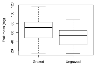
If we plot the distribution of fruit mass in the two groups we see that the distributions are consistent with the analytical results. Grazed plants have a higher average fruit production than do ungrazed plants.

Fig. 1  The effect of grazing on fruit mass

So far we've been ignoring the covariate root size that was also measured as part of the experiment. In Fig. 2 I plot fruit mass versus root size color coding the points according to their grazing status. I use the numeric values of the Grazing factor, 1 and 2, as the argument to col= to specify the color codes 1 and 2. I do the same to get different plotting symbols but this time using 1 and 2 to select either the first or the second element of the vector mypch that specifies open and filled circles.

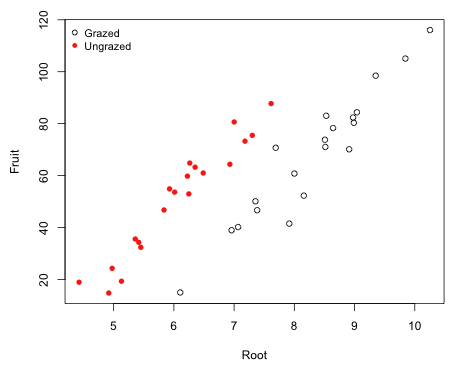
Fig. 2  The effect of grazing on fruit mass while controlling for root size

Observe that the root size distributions are different in the two treatment groups. The plants in the grazed group tend to have larger root sizes that those in the ungrazed group. Also notice that there is a strong linear relationship between fruit production and root size. Thus it seems possible that by not accounting for root size in our analysis that the estimation of a treatment effect has been compromised.

A poor way to control for root size—create a ratio variable

In the biological literature a method that is often used to adjust for a potentially confounding variable such as root size is to create a new response variable that is the ratio of the original response variable and the confounder. Using this approach here we would analyze the ratio of fruit production to root size rather than fruit production. If we do so we find that the fruit production to root size ratio is not significantly different between the two grazing groups.

Response: Fruit/Root
          Df  Sum Sq Mean Sq F value Pr(>F)
Grazing    1   0.177  0.1773  0.0306  0.862
Residuals 38 219.994  5.7893              

Residuals:
    Min      1Q  Median      3Q     Max
-5.4980 -1.6605  0.7814  1.5884  3.4426

Coefficients:
                Estimate Std. Error t value Pr(>|t|)   
(Intercept)       7.9464     0.5380  14.770   <2e-16 ***
GrazingUngrazed   0.1332     0.7609   0.175    0.862   
---
Signif. codes:  0 ‘***’ 0.001 ‘**’ 0.01 ‘*’ 0.05 ‘.’ 0.1 ‘ ’ 1

Residual standard error: 2.406 on 38 degrees of freedom
Multiple R-squared: 0.0008054,     Adjusted R-squared: -0.02549
F-statistic: 0.03063 on 1 and 38 DF,  p-value: 0.862

Notice that although the point estimate of the grazing effect on the ratio is not significant, it is positive suggesting that ungrazed plots have a larger fruit to root ratio than do grazed plots. This is the reverse of the direction we found when not accounting for root size.

In addition to creating a variable that is harder to interpret than the original variable, the use of a ratio response makes some unwarranted assumptions about the relationship of fruit production to root size. We'll examine these assumptions below after we consider a better way to adjust for root size—analysis of covariance.

A better way to control for root size—analysis of covariance

Notice that in Fig. 2 the two treatment groups are completely segregated each lying within a distinct band. At any root size where the treatment groups overlap, the fruit production is seen to be higher for the ungrazed group and than for the grazed group. This suggests that there is a treatment effect, although not as simple as an ordinary mean difference between the groups. Given that a linear relationship between fruit mass and root size appears to be appropriate for both treatment groups there are three possible models to consider here.

• Model 1: Single line model. Fruit production is linearly related to root size. Grazing has no effect (Fig. 3a).
• Model 2: Parallel lines model, also called the additive model. Fruit production is linearly related to root size and the relationship is the same under both grazing regimes. The effect of grazing is to decrease fruit production by a constant amount at all root sizes (Fig. 3b). This is the classic analysis of covariance model and appears to match what we see in Fig. 2.
• Model 3: Non-parallel lines model, also called the interaction model. Fruit production is linearly related to root size but the nature of the relationship changes depending on the presence or absence of grazing (Fig. 3c).

(a)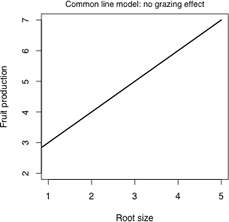	(b)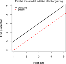	(c)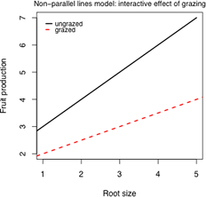
Fig. 3  Three possible regression models for the effect of grazing on fruit production

Let

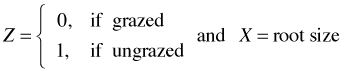
The three models can be expressed as follows.

Regression models with categorical variables can also be written as multiple linear equations where there is a separate equation for each category of the categorical variable. A regression model with a single dummy variable yields two different equations, one for each value of the dummy variable. To see the connection between the three models described above and Fig. 3, replace the dummy variable Z by its values 0 and 1.

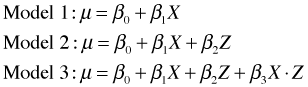
Model 2: Parallel lines

We have the equations of two lines that have the same slope, β₁, but different intercepts. The parameter β₂ measures how much the intercepts differ. It also corresponds to the vertical distance between the parallel lines in Fig. 3b.

Model 3: Non-parallel lines

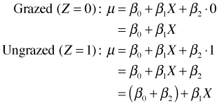
Here we have the equations of two lines with different intercepts and different slopes. The parameter β₂ measures how much the intercepts differ. The parameter β₃ measures how much the slopes differ.

I fit a sequence of models starting with the single line model, then the additive model, and finally the full interaction model. The additive model is the analysis of covariance model in this example. When we examine model 1 in which root is the only predictor, we see that there is a significant positive effect due to root size.

Next we turn to model 2, the parallel lines model.

Response: Fruit
          Df  Sum Sq Mean Sq F value    Pr(>F)   
Root       1 16795.0 16795.0  368.91 < 2.2e-16 ***
Grazing    1  5264.4  5264.4  115.63 6.107e-13 ***
Residuals 37  1684.5    45.5                     
---
Signif. codes:  0 ‘***’ 0.001 ‘**’ 0.01 ‘*’ 0.05 ‘.’ 0.1 ‘ ’ 1

From the output we see that having controlled for root size, there is a significant grazing effect on fruit production. To see the nature of that effect we can examine the summary table of the model.

Residuals:
     Min       1Q   Median       3Q      Max
-17.1920  -2.8224   0.3223   3.9144  17.3290

Coefficients:
                Estimate Std. Error t value Pr(>|t|)   
(Intercept)     -127.829      9.664  -13.23 1.35e-15 ***
Root              23.560      1.149   20.51  < 2e-16 ***
GrazingUngrazed   36.103      3.357   10.75 6.11e-13 ***
---
Signif. codes:  0 ‘***’ 0.001 ‘**’ 0.01 ‘*’ 0.05 ‘.’ 0.1 ‘ ’ 1

Residual standard error: 6.747 on 37 degrees of freedom
Multiple R-squared: 0.9291,            Adjusted R-squared: 0.9252
F-statistic: 242.3 on 2 and 37 DF,  p-value: < 2.2e-16

According to model 2 the fruits of ungrazed plants are on average 36.1 mg heavier than the fruits of grazed plants. Finally I consider model 3, the non-parallel lines model.

Response: Fruit
             Df  Sum Sq Mean Sq  F value    Pr(>F)   
Root          1 16795.0 16795.0 359.9681 < 2.2e-16 ***
Grazing       1  5264.4  5264.4 112.8316 1.209e-12 ***
Root:Grazing  1     4.8     4.8   0.1031      0.75   
Residuals    36  1679.6    46.7                      
---
Signif. codes:  0 ‘***’ 0.001 ‘**’ 0.01 ‘*’ 0.05 ‘.’ 0.1 ‘ ’ 1

The interaction is not significant thus we can stick with the parallel lines model. Because the interaction is not significant, the linear relationship between fruit mass and root size is the same in both grazing groups. I re-examine the coefficients of the parallel lines model.

The parallel lines model is the classic analysis of covariance model. In this model the grazing effect term adds to the intercept, so the intercept of the fruit-root relationship is 36.1 units larger for ungrazed plants than it is for grazed plants. Because the lines are parallel, 36.1 is also the vertical distance between the lines at any root size. So we can say that ungrazed plants yield fruit that is on average 36.1 mg heavier than the the fruit of grazed plants after controlling for the size of the plant (based on the size of their root). This result is the exact opposite of the one we obtained when we did not control for the confounding effects of root size. The utility of the analysis of covariance model is that it allows us to statistically control for systematic differences between groups so that we can validly compare the means of the groups.

Graphing the analysis of covariance model

I graph the raw data and superimpose the best model, the parallel lines model (model 2). A convenient way to superimpose functions on already plotted data is with the curve function. The first argument of curve should be a function of the variable x. To force the curve function to add the graph of the function to the currently active graphics window we need to include the add=T argument.

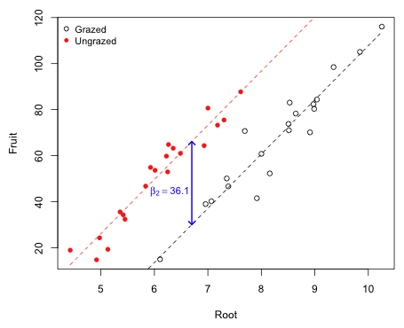
Fig. 4  Analysis of covariance model showing the treatment effect β₂

The estimate of the grazing effect on fruit mass corresponds to the vertical distance between the parallel lines in Fig. 4. Generally speaking when graphing regression lines we should not extrapolate beyond the range of the data. I redraw Fig. 4 and truncate the regression lines accordingly using the minimum and maximum values of root size in each grazing group. The curve function has from= and to= arguments that allow you to specify x-axis limits in drawing the function.

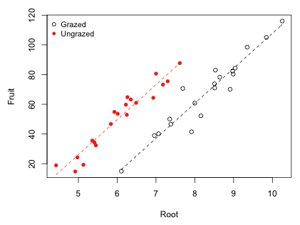
Fig. 5  Analysis of covariance model with regression lines truncated to the range of data

The problem with ratios

Having adjusted for root size by using the analysis of covariance model let's revisit the regression model that used the ratio of fruit mass to root size as the response variable and see what's wrong with it. If Y is fruit mass, X is root size, and Z is a dummy variable indicating grazing status, then the regression model we fit for the ratio of fruit mass to root size is the following.

where . I've used different symbols for the regression coefficients so as not to confuse them with the analysis of covariance model above. Multiply both sides of the equation by X, the root size variable.

where ε* is just my notation for the new error term. (Note: Because ε is multiplied by X this model assumes that the standard deviation of the residuals is not constant but varies with the magnitude of X. So, we have a heteroscedastic error model.) Compare this last equation with model 3, the non-parallel lines model, described above.

There are two obvious differences between the models shown in eqns (2) and (3).

1. The first and third terms on the right side of eqn (3) are missing in the ratio model of eqn (2). These terms together define the intercepts of the two lines that correspond to the two grazing treatments. Because the term β₂Z is missing in eqn (2) the ratio model assumes the intercepts in a plot of Y versus X are the same for the two grazing treatments. Because β₀ is also missing in eqn (2) the ratio model assumes that both of the intercepts are zero! At first glance this may not seem unreasonable, after all if the root size is zero then the fruit production should also be zero. But the ratio model is actually making a far bigger assumption here. It assumes that the linear relationship that is apparent in Fig. 2 extends beyond the range of the data all the way to the origin. We have no evidence of that. All we know for sure is that over the range of the data, for which the root size is between 5 and 10, the relationship appears to be linear. Over the root size range from 0 to 10 the relationship could be curvilinear.
2. In the ratio model of eqn (1) a treatment difference corresponds to γ₁ ≠ 0. But in eqn (2) we see that γ₁ causes the slope of the fruit mass to root size relationship to be different depending on the grazing treatment. Thus when we fit a ratio model and look for a treatment effect we're testing for a difference in these slopes. In the analysis of covariance model the slopes need to be the same in the two treatment groups for the notion of a treatment effect to make sense. (We tested for this by fitting the interaction model and verifying that the interaction is not significant.). When the slopes are the same the effect of grazing on fruit production is the same regardless of the size of the plant. The treatment effect is the vertical distance between the lines. So the ratio model and the analysis of covariance find a "treatment effect" in completely different portions of the fruit mass versus root size linear relationship. For the ratio model a treatment effect is a difference in slopes. For the analysis of covariance model a treatment effect is a difference in intercepts (after verifying that the slopes are the same). If the slopes are not the same in the analysis of covariance model then there is not a fixed treatment effect; it varies with root size.

Fig. 6 shows the analysis of covariance model of Fig. 4 and superimposes the ratio model of eqn (2) using the coefficients estimated from eqn (1). The badness of the ratio model is readily apparent.

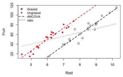
Fig. 6  Analysis of covariance model compared with ratio regression model

Fig. 6 is a bit unfair because fitting the ratio model in eqn (1) using least squares does not yield the same parameter estimates as fitting eqn (2) using least squares (although they are close). Basically the difference is that the mean of a ratio is not equal to the ratio of the means. Still dividing a response variable by a covariate as an attempt to "standardize" it is generally a bad idea. Ratio variables cause problems in ordinary regression because their distribution is typically non-normal. Even worse the use of ratios has the potential of inducing spurious correlations between the variables of interest. Recognition of the problems posed by ratio variables dates back to the beginning of statistics itself (Pearson 1897). Over the years researchers in applied disciplines have repeatedly "rediscovered" the ratio problem. Some recent criticisms of using ratio variables in regression instead of analysis of covariance, organized by discipline, include the following.

• aquatic science: Jackson et al. (1990)
• conservation biology: Riggs et al. (2008), Serrano et al. (2008)
• ecology: Beaupre and Dunham (1995), Packard and Boardman (1988), Jackson and Somers (1991), Jasienski and Bazzaz (1999)
• environmental science: McCuen and Surbeck (2008), Righetti et al. (2012)
• horticulture: Righetti et al. (2007)
• medicine: Allison et al. (1995), Tu et al. (2004), Tu et al. (2010)
• physiology: Tanner (1949), Horton and Redak (1993), Poehlman and Toth (1995), Packard and Boardman (1999), Raubenheimer and Simpson (1992), Karp et al. (2012)
• psychology: Porter and Raudenbush (1987)
• sociology and political science: Chilton (1982), Logan (1982), Kritzer (1990)
• statistics: Kronmal (1993)
• systematics: Atchley et al. (1976)

Here are two excerpts of the criticisms found in these papers. From Beaupre and Dunham (1995), p. 880:

(The) dangers (of using ratios) include: (1) identification of spurious relationships which may lead to erroneous biological interpretation, (2) false identification of effects as significant, (3) failure to identify significant effects and (4) potentially large errors in ... estimation.

… We believe that our reanalysis suggests that these problems are far worse than most appreciate. We urge physiologists to abandon analyses of ratio-based indices in favour of ANCOVA.

From Packard and Boardman (1999), p. 1:

Ecological physiologists commonly divide individual values for variables of interest by corresponding measures for body size to adjust (or scale) data that vary in magnitude or intensity with body size of the animals being studied. These ratios are formed in an attempt to increase the precision of data gathered in planned experiments or to remove the confounding effects of body size from descriptive studies...

This procedure for adjusting data is based on the implicit, albeit critical, assumption that the variable of interest varies isometrically with body size. Isometry occurs whenever a plot of a physiological variable (y) against a measure of body size (x) yields a straight line that passes through the origin of a graph with linear coordinates. Alternatively allometry obtains whenever such a plot yields either a curved line or a straight line that intersects the Y-axis at some point other than zero. Most physiological variables change allometrically with body size (Smith 1984), so the assumption of isometry that is fundamental to the use of ratios for scaling data seldom is satisfied ... statistical analyses of ratios lead  to conclusions that are inconsistent with impressions gained from visual examinations of data displayed in bivariate plots. In comparison, analyses of covariance lead to conclusions that agree with impressions gained from these same plots. We therefore recommend that ecological physiologists discontinue using ratios to scale data and that they use the ANCOVA instead.

The opinion of all of these authors is that ratios should almost never be used for statistical control purposes. Their most important objection is that ratios can correctly adjust for the effect of the covariate only when the the response and the covariate are collinear with an intercept of zero. If the intercept is not zero or the relationship is nonlinear (or linear only over a short range), regression with a ratio response can yield spurious results. While the use of ratios is not always inappropriate, if the ratio itself is not of primary interest but is being used only to adjust the value of the response, then analysis of covariance is a far better approach.

Comparing regression models across groups

Forrester and Steele (2004) studied the effect of competition and resource availability on the mortality of gobies. Resource availability for gobies was defined to be the density of available refuges that allow gobies to hide from their potential predators. It is expected that mortality will increase as population density increases because of intraspecific competition for refuges. Because each refuge is only used by a single goby, the effect of increasing population density should be lower when the availability of refuges is high. The experiment was conducted in the natural habitat of gobies where refuge density was classified into three categories: low, medium, and high. Six replicates of each of these refuge density categories were obtained and for each replicate a different goby density was maintained. Using a detailed census of the resident fish population, mortality was recorded as percent survival. Because percentages are bounded on the interval 0 to 100 treating them as normally distributed variables can lead to nonsensical results. Forrester and Steele (2004) chose to ignore these complications and for today's lecture we will too.

Unlike the Ipomopsis example considered previously where the focus was to compare means across groups and regression was used only to account for a confounding variable, here the focus is on the regression equation itself. The question of interest is whether the relationship between goby mortality and goby density is different for different categories of refuge density. In the Ipomopsis example we had to first rule out the presence of an interaction between the continuous predictor "root" and the categorical treatment variable "grazing" in order to estimate a treatment effect. In the goby experiment the interaction between the continuous predictor goby density and the categorical predictor refuge density was the focus of the analysis. If a significant interaction is present it means that the relationship between goby mortality and goby density is different for different refuge densities.

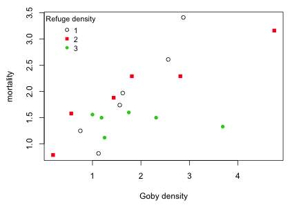
Fig. 7  Effect of goby density and refuge density on goby mortality

The graph would seem to indicate that the goby mortality-goby density relationship varies with refuge density. I fit a model that includes an interaction between refuge density and goby density.

The interaction is statistically significant. The regression equation that was fit is the following. If x = goby density,

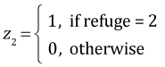, and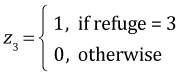 

then the predicted mean is

This reduces to three regression models, one for each refuge type.

refuge	z1	z2
1	0	0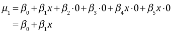
2	1	0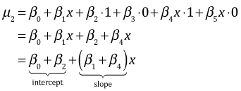
3	0	1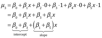

Next we examine the summary table of the model.

Residuals:
     Min       1Q   Median       3Q      Max
-0.47439 -0.10553  0.06187  0.15585  0.35897

Coefficients:
                        Estimate Std. Error t value Pr(>|t|)   
(Intercept)               0.0843     0.3009   0.280 0.784129   
density                   1.0756     0.1581   6.805 1.89e-05 ***
factor(refuge)2           1.0493     0.3564   2.944 0.012288 * 
factor(refuge)3           1.4016     0.4021   3.486 0.004500 **
density:factor(refuge)2  -0.6269     0.1762  -3.558 0.003938 **
density:factor(refuge)3  -1.1029     0.2035  -5.419 0.000155 ***
---
Signif. codes:  0 ‘***’ 0.001 ‘**’ 0.01 ‘*’ 0.05 ‘.’ 0.1 ‘ ’ 1

Residual standard error: 0.2901 on 12 degrees of freedom
Multiple R-squared: 0.8867,  Adjusted R-squared: 0.8395
F-statistic: 18.78 on 5 and 12 DF,  p-value: 2.664e-05

From the summary table we see that β₄ ≠ 0 (p = .004) so the slopes for refuge =1 and refuge = 2 differ. Because the point estimate of β₄ is negative, the slope for refuge 2 is less than the slope for refuge = 1. Also from the summary table we see that β₅ ≠ 0 (p = .0002) so the slopes for refuge =1 and refuge = 3 differ. Because the point estimate of β₅ is negative, the slope for refuge = 3 is less than the slope for refuge = 1.

To compare the slopes for refuge = 2 and refuge =3 we can refit the model choosing a different reference level for refuge. I make refuge = 3 the reference level in the run below.

Residuals:
     Min       1Q   Median       3Q      Max
-0.47439 -0.10553  0.06187  0.15585  0.35897

Coefficients:
                                      Estimate Std. Error t value Pr(>|t|)   
(Intercept)                            1.48587    0.26674   5.571 0.000122 ***
density                               -0.02728    0.12818  -0.213 0.835038   
factor(refuge, levels = 3:1)2         -0.35231    0.32811  -1.074 0.304049   
factor(refuge, levels = 3:1)1         -1.40157    0.40211  -3.486 0.004500 **
density:factor(refuge, levels = 3:1)2  0.47603    0.14996   3.174 0.008003 **
density:factor(refuge, levels = 3:1)1  1.10292    0.20351   5.419 0.000155 ***
---
Signif. codes:  0 ‘***’ 0.001 ‘**’ 0.01 ‘*’ 0.05 ‘.’ 0.1 ‘ ’ 1

Residual standard error: 0.2901 on 12 degrees of freedom
Multiple R-squared: 0.8867,  Adjusted R-squared: 0.8395
F-statistic: 18.78 on 5 and 12 DF,  p-value: 2.664e-05

With refuge = 3 as the reference level, a test of H₀: β₄ = 0 is a test of whether the slopes for refuge = 2 and refuge = 3 are the same. From the output we conclude β₄ ≠ 0 (p = 0.008). The point estimate is positive so we conclude that the slope for refuge = 2 exceeds the slope for refuge = 1.

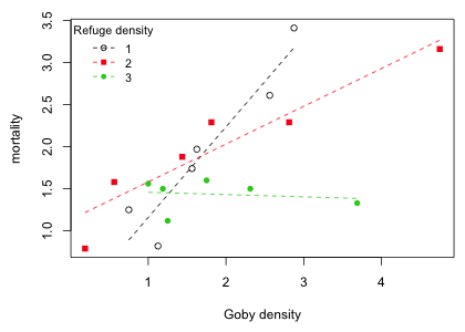
To graph the model we can use the abline function applied to lm models fit separately for different values of refuge. The abline extracts the intercept and slope form the lm model object and draws the regression line.

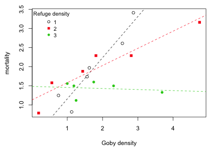
Fig. 8  Regression of mortality on goby density separately by range density

Alternatively we can produce Fig. 8 by extracting the intercepts and slopes ourselves from the full interaction model and then providing them to abline to plot the lines.

Unfortunately abline does not have an option that permits restricting the regression line to the range of the data. For that we could use the curve function like we did in Fig. 5 for the Ipomopsis example. Alternatively we can use the predict function with the newdata argument to obtain the coordinates of the endpoints of the regression line. The range function can be used to calculate the minimum and maximum values of goby density for a given refuge category and the predict function used to obtain the model predictions at those values. I assemble all of this as a function whose sole argument is the refuge density category.

Using the function I add the regression lines to a scatter plot of the data.

Fig. 9   Regression of goby mortality on goby density separately by refuge density in which regression lines are restricted to the range of the data

Assessing treatment differences in the presence of an interaction

If we attempt to use analysis of covariance to control for a continuous covariate and it turns out that there is a significant interaction between the treatment and the covariate then there is no unique treatment effect. The magnitude (and perhaps the direction) of the treatment effect varies with the value of the continuous covariate. So, in this case we might just summarize the results by reporting the different slopes of the regression lines for the different treatments. Still, we might be interested in knowing if there is a range of covariate values for which a significant treatment effect did occur and perhaps obtain a ranking of the treatments over that range. For example, in Fig. 9 it appears that on the left side of the diagram refuge density doesn't matter, but on the right side of Fig. 9 the percent mortality for different values of refuge can be ranked as follows: mortality(refuge = 1) > mortality(refuge = 2) > mortality(refuge = 3). Can we quantify this result and perhaps summarize it graphically?

Using the trick that was discussed previously, I begin by reparameterizing the model so that the parameter estimates we obtain are estimates of the individual slopes and intercepts.

Residuals:
     Min       1Q   Median       3Q      Max
-0.47439 -0.10553  0.06187  0.15585  0.35897

Coefficients:
                        Estimate Std. Error t value Pr(>|t|)    
factor(refuge)1          0.08430    0.30090   0.280 0.784129   
factor(refuge)2          1.13355    0.19108   5.932 6.90e-05 ***
factor(refuge)3          1.48587    0.26674   5.571 0.000122 ***
density:factor(refuge)1  1.07564    0.15807   6.805 1.89e-05 ***
density:factor(refuge)2  0.44875    0.07782   5.767 8.93e-05 ***
density:factor(refuge)3 -0.02728    0.12818  -0.213 0.835038   
---
Signif. codes:  0 ‘***’ 0.001 ‘**’ 0.01 ‘*’ 0.05 ‘.’ 0.1 ‘ ’ 1

Residual standard error: 0.2901 on 12 degrees of freedom
Multiple R-squared: 0.985,   Adjusted R-squared: 0.9775
F-statistic: 131.2 on 6 and 12 DF,  p-value: 3.13e-10

Based on the labels of the coefficient vector of regression parameters I write a function that constructs the appropriate vector of regressors corresponding to the given values of density and refuge.

Our goal is to calculate the confidence level that allows individual overlapping confidence intervals to be used to graphically assess treatment differences separately at each value of goby density. To accomplish this we need the ci.func function that was first presented in lecture 5.

This function requires the variance-covariance matrix of the means. I illustrate how to create it for the smallest goby density when refuge = 1.

I build a data frame consisting of the three values of refuge density with goby density = 1.125.

I construct a vector of regressors for each of the three observations in the data frame and assemble them in a matrix.

I obtain the variance-covariance matrix of the means and use it as input to the ci.func function to obtain the difference-adjusted confidence levels needed to make pairwise comparisons between the three refuge category means.

I assemble the above steps in a function so that we can obtain the difference-adjusted confidence levels using any goby density value.

Finally I use this function on each of the different goby density values using sapply to apply the function separately to each density value.

The range of confidence levels reported is from 0.85 to 0.87 so there isn't much variability. Clearly we can get by with using just one value. I add 95% and 85% confidence intervals for the mean to each point on the regression line that corresponds to an observed goby density. To illustrate the steps I start by doing just refuge = 1.

Using the means and standard errors I plot the regression line, 95% confidence intervals of the mean at each goby density value for refuge = 1, and the 85% difference-adjusted intervals.

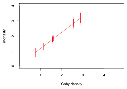Fig. 10   Preliminary graph showing confidence intervals for refuge = 1

Finally I assemble things as a function whose argument is the value of refuge. I include two color arguments to specify colors for the regression line and the difference-adjusted confidence levels.

Finally I draw the graph.

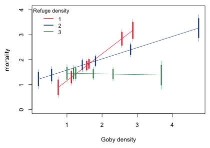Fig. 11  Graph to compare mean mortality across refuge level for specific values of goby density

What we can see from Fig. 11 is that when goby density > 1.8 (approximately) refuge = 3 has a significantly lower mean mortality than do the other two values of refuge. The sparse data make it difficult to determine these change point precisely but probably when goby density > 2.8, refuge = 2 has a significantly lower mortality than does refuge = 1.

Cited references

• Crawley, Michael J. 2002. Statistical Computing: An Introduction to Data Analysis Using S-Plus. Wiley, New York.
• Crawley, Michael J. 2007. The R Book. Wiley, New York.
• Forrester, G. E. and M. A. Steele. 2004. Predators, prey refuges, and the spatial scaling of density-dependent prey mortality. Ecology 85: 1332–1342.

References on the ratio "problem"

• Allison, D. B., F. Paultre, M. I. Goran, E. T. Poehlman, and S. B. Heymsfield. 1995. Statistical considerations regarding the use of ratios to adjust data. International Journal of Obesity 19: 644–652.
• Atchley, W. R., C. T. Gaskins, and D. Anderson. 1976. Statistical properties of ratios. I. Empirical results. Systematic Zoology 25: 137–148.
• Beaupre, S. J. and A. E. Dunham. 1995. A comparison of ratio-based and covariance analyses of a nutritional data set. Functional Ecology 9: 876–880.
• Chilton, R. 1982. Analyzing urban crime data: deterrence and the limitations of arrests per offense ratios. Criminology 19: 590–607.
• Horton, D. R. and R. A. Redak. 1993. Further comments on analysis of covariance in insect dietary studies. Entomologia Experimentalis Et Applicata. 69: 263–275.
• Jackson, D. A., H. H. Harvey, K. M. Somers. 1990. Ratios in aquatic sciences: Statistical shortcomings with mean depth and the morphoedaphic index. Canadian Journal of Fisheries and Aquatic Sciences 47: 1788–1795.
• Jackson, D. A. and K. M. Somers. 1991. The spectre of 'spurious' correlations. Oecologia 86: 147–151.
• Jasienski, M. and F. A. Bazzaz. 1999. The fallacy of ratios and the testability of models in biology. Oikos 84: 321–326.
• Karp, N. A., A. Segonds-Pichon, A. K. B. Gerdin, R. Ramirez-Solis, and J. K. White. 2012. The fallacy of ratio correction to address confounding factors. Laboratory Animals 46: 245–252.
• Kritzer, H. M. 1990. Substance and method in the use of ratio variables, or the spurious nature of spurious correlation? The Journal of Politics 52: 243–254.
• Kronmal, R. A. 1993. Spurious correlation and the fallacy of the ratio standard revisited. Journal of the Royal Statistical Society Series A: Statistics in Society 156: 379–392.
• Logan, C. H. 1982. Problems in ratio correlation: the case of deterrence research. Social Forces 60: 791–810.
• McCuen, R. H. and C. Q. Surbeck. 2008. An alternative to specious linearization of environmental models. Water Research 42: 4033–4040.
• Packard, G. C. and T. J. Boardman. 1988. The misuse of ratios, indices, and percentages in ecophysiological research. Physiological Zoology 61: 1–9.
• Packard, G. C and T. J. Boardman. 1999. The use of percentages and size-specific indices to normalize physiological data for variation in body size: wasted time, wasted effort? Comparative Biochemistry and Physiology A—Molecular and Integrative Physiology 122(1): 37–44.
• Pearson, K. 1897. Mathematical contributions to the theory of evolution-on a form of spurious correlation which may arise when indices are used in the measurements of organs. Proceedings of the Royal Society of London 60: 489–497.
• Poehlman, E. T. and M. J. Toth. 1995. Mathematical ratios lead to spurious conclusions regarding age-related and sex-related differences in resting metabolic rate. American Journal of Clinical Nutrition 61: 482–485.
• Porter, A. C. and S. W. Raudenbush. 1987. Analysis of covariance: its model and use in psychological research. Journal of Counseling Psychology 34(4): 383–392.
• Raubenheimer, D. and S. J. Simpson. 1992. Analysis of covariance: an alternative to nutritional indices. Entomologia Experimentalis Et Applicata 62: 221–231.
• Riggs, M. R., K. J. Haroldson, and M. A. Hanson. 2008. Analysis of covariance models for data from observational field studies. Journal of Wildlife Management 72: 34–43.
• Righetti, T. L., D. R. Sandrock, B. Strik, C. Vasconcelos, Y. Moreno, S. Ortega-Farias, and P. Banados. 2007. Analysis of ratio-based responses. Journal of the American Society for Horticultural Science 132: 3–13.
• Righetti, T. L., D. Dalthorp, J. Lambrinos, B. Strik, D. Sandrock, and C. Phillips. 2012. International Journal of Environmental Analytical Chemistry 92: 1–27.
• Serrano, E., R. Alpizar-Jara, N. Morellet, and A. J. M. Hewison. 2008. A half a century of measuring ungulate body condition using indices: is it time for a change? European Journal of Wildlife Research 54(4): 675–680.
• Tanner, J. M. 1949. Fallacy of per-weight and per-surface area standards, and their relation to spurious correlation. Journal of the Applied Physiology 2: 1–15.
• Tu, Y.-K., V. Clerehugh, and M. S. Gilthorpe. 2004. Ratio variables in regression analysis can give rise to spurious results: illustration from two studies in periodontology. Journal of Dentistry 32: 143–151.
• Tu, Y.-K. , G. R. Law, G. T. H. Ellison, and M. S. Gilthorpe. 2010. Ratio index variables or ANCOVA? Fisher’s cats revisited. Pharmaceutical Statistics 9: 77–83

R Code

A compact collection of all the R code displayed in this document appears here.

Course Home Page