Lecture 8—Wednesday, September 19, 2012

Topics

• Obtaining the variance-covariance matrix for means
  • A shortcut for obtaining the variance-covariance matrix of the means
  • Using the estimates of the effects to obtain the variance-covariance matrix of the means
• Calculating difference-adjusted confidence intervals for the treatment means
• Creating an interaction plot using the lattice package
  • Group panel function
  • Prepanel function
  • Drawing the graph
  • Adding a key
  • Improving the display with the latticeExtra package
• R code

R functions and commands demonstrated

• panel.superpose (from lattice) is the panel function used with groups to indicate that individual groups are to be distinguished within panels. It can be used with a user-specified panel.groups function for customized displays.
• useOuterStrips (from latticeExtra) can be used to place panels on the left edge and the top edge of panel graphs.

R function options

• group.number is a key word available in lattice for identifying the observations that are being used in the current group.
• groups= (argument to lattice functions) defines the grouping variable in lattice graphs. Grouping variables affect the display in a single panel while conditioning variables affect the display in different panels.
• prepanel= (argument to xyplot) identifies a user-defined prepanel function that determines the x- and/or y-limits for individual panels.

Additional R packages used

• lattice for the xyplot function.
• latticeExtra for the useOuterStrips function.
• lme4 for the lmer function.

Obtaining the variance-covariance matrix for means

I refit the model we ended with last time: a 4-factor model consisting of a two-factor interaction, two additional main effects, and crossed random effects that describe variability across blocks and species.

The goal today is to produce a single graph that summarizes the treatment structure of this experiment. The centerpiece for the graphical display will be a depiction of the two-factor interaction between lh and n separately for different levels of func and p. The main effects of func and p will serve to shift this interaction vertically along the y-axis yielding four identical two-factor interaction diagrams. Because the main effects of func and p are statistically significant the individual means on different two-factor interactions diagrams will be significantly different from each other. Thus in constructing the graph we can focus on pairwise differences between the means on a single interaction diagram. To summarize the pairwise differences we'll superimpose difference-adjusted confidence intervals for individual means on top of the interaction diagram. To do this we'll need to obtain the variance-covariance matrix of the means.

A shortcut for obtaining the variance-covariance matrix of the means

The vcov function when applied to a model returns the variance-covariance matrix of the parameter estimates.

The parameter estimates here are effect estimates, not individual treatment means. For certain models it is possible to force R to reparameterize the model so that it returns cell means rather than effect estimates. It is not possible to do this with the model currently under consideration, but if the model were slightly simpler we could. Suppose the final model consisted only of the two factor interaction between lh and n.

If we replace the term factor(lh)*factor(n) with the expression factor(lh):factor(n)-1, the parameters that R returns are the treatment means. This expression appears to fit a model with an interaction but without main effects and an intercept. Rather than fit such a silly model R instead estimates each category of the interaction term separately replacing the intercept and main effects with the separate category estimates. We still get four parameters but now instead of obtaining a mean and three effect estimates we obtain four treatment means.

The vcov function applied to this model yields the variance-covariance matrix of the means.

If our model consisted of only a single factor, say lh, then removing the intercept from this model would cause R to estimate the treatment means at both levels of lh.

The vcov function applied to this model yields the variance-covariance matrix of the means.

Using the estimates of the effects to obtain the variance-covariance matrix of the means

The shortcut method won't work for the current model because it is too complicated. We'll need to construct a contrast matrix C such that when multiplied by the vector of regression parameter estimates it returns the treatment means for the treatments of interest. We've done this previously and the same approach will work here. The only difference is that we're working with a model estimated by lmer rather than by lm. We need to write a function that generates the values of the dummy variables in the same order as the coefficients estimated by lmer. To see this order I examine the names of the coefficient estimates and construct a function whose arguments are the values of the four factors.

I construct a matrix that contains all the possible combinations of the values of lh and n.

I specify the values func = 'inoc' and p = 0 and evaluate the function separately on the rows of this matrix by using the apply function. Because apply extracts each row of the matrix as a vector (each a vector of length 2) I reformulate the function cmat2 as a generic function in which the first two arguments are elements 1 and 2 of a vector.

The contrast matrix we need is the transpose of this matrix.

Finally I set this up as a function with arguments func and p.

I use the function to calculate the treatment means and the variance-covariance matrix of the means for func = 'inoc' and p = 0.

Calculating difference-adjusted confidence intervals for the treatment means

To obtain the confidence level for the precision-based confidence intervals we need to modify the function we used previously. That function used a t-distribution with the residual degrees of freedom from the model as the multiplier. As was discussed in lecture 6 the determination of degrees of freedom in mixed effects models is problematic. Instead we'll assume that a normal distribution is an adequate substitute. I replace the occurrences of qt and pt with qnorm and pnorm respectively and remove the degrees of freedom argument. I also eliminate the second argument of the ci.func function. This was the fitted regression model, which was used only to extract the degrees of freedom for the t-distribution.

We have four means so the first argument to this function is 1:4. If I use the function on the variance-covariance matrix vmat we calculated above R issues an error message.

The problem appears to be that the pnorm and qnorm functions don't recognize the class of vmat, "dgeMatrix", that it inherited from the lme4 package. If I use the as.matrix function to change the class of vmat to "matrix" the function works.

When I try the function on a different variance-covariance matrix obtained with different choices for func and p, I get slightly different results.

These differences are probably not large enough to matter but I elect to obtain separate confidence levels for each of the combinations of func and p anyway. To this end I write a function that obtains the difference-adjusted confidence levels, calculates the 95% and difference-adjusted confidence intervals, and assembles them along with the means and the appropriate labels in a data frame. In the function I use the lowest difference-adjusted confidence level that was obtained for all the comparisons. It turns out that if we repeat this using the largest calculated confidence level the conclusions we would draw from the graph don't change.

Finally I use the function separately for the four different combinations of func and p and assemble the results in a single data frame.

Creating an interaction plot using the lattice package

Previously we created an interaction plot using base graphics. Here I illustrate doing the same using the lattice package. While we could do something similar to what we did before where we subsetted the data and first drew one profile then the other, it is far more efficient to use the groups argument in lattice. We've use it previously to obtain different colors and symbol types when plotting different groups. We can do more elaborate things separately by group if we create our own group panel function.

Group panel function

When the groups argument is included lattice calls a specific panel function called panel.superpose. The panel.superpose function in turn calls something called a panel.groups function that by default is panel.xyplot in which the points are colored separately by group. To draw the error bars we will need to create our own customized panel.groups function. Here's the function I created followed by an explanation of the various parts of the code.

I pass to the group panel function the colors and plot characters I want it to use for the groups (the col and pch arguments in the function definition). The subscripts argument was explained previously and will be used to get the correct observations for use in the current panel for variables that were not included in the original function call. Notice the ... notation that appears in a couple of places. It's used so that any additional arguments that lattice would normally need in displaying groups get passed to the appropriate functions. One new argument is group.number. It records the number of the group currently being drawn. It will have the value 1 or 2 here because there are only two groups.

The first four lines of the function use the subscripts variable to select the confidence bounds that are appropriate for the panel currently being drawn. When the panel function is called upon to draw a panel the variable subscripts identifies the observations whose values of func and p (the variables that defines the panels) are being used for the current panel. So, in the above code the expressions fac.vals$low95[subscripts] and fac.vals$up95[subscripts] extract a vector of lower 95% endpoints and a vector of upper 95% endpoints corresponding to the level of the conditioning variable that is currently being plotted. This is also the role the notation x and y have in the function. By default each time a panel is drawn the correct set of lh and est values (the x and y variables) are selected. Because low95, up95 , low85, and up85 are not part of the original function call we have to extract the correct set of observations for the panel ourselves.

The myjitter variable denotes the amount I want to shift the error bars for the two profiles. The col2 variable contains the colors for the difference-adjusted confidence intervals. The panel.arrows and panel.segments functions are just the lattice version of the arrows and segments functions of base graphics. Notice how I use the group.number variable to select the correct value for myjiitter and the correct color for the difference-adjusted error bars for the current group being plotted.

Prepanel function

Ordinarily lattice uses the variables in the main function call to determine the appropriate x-limits and y-limits of the graph. We've previously overridden this choice by specifying the xlim and ylim arguments, which forces the limits in all the panels to be the same. If we would like the limits to potentially vary between panels we can supply a prepanel function in which we pass to it those variables that are needed to calculate the correct limits. Below is a prepanel function that uses the values of the variables y, ly, and uy to reset the limits on the y-axis. Its return value is the new setting of ylim for the panel currently being drawn.

In the function call I will specify uy and ly to be the variables containing the upper 95% and lower 95% confidence bounds.

Drawing the graph

The call to lattice to produce the graph is shown below.

• The summation expression after the vertical bar defines the panels. In this case func+factor(p, level=0:1, labels=paste('P = ', 0:1, sep='')) will cause the panels to be defined by all combinations of the levels of func and p.
• In the conditioning expression I explicitly declare p to be a factor in order to create more informative labels for the factor levels: "P = 0" and "P = 1".
• groups = factor(n) declares the levels of n as defining the groups.
• col=c(2,1) and pch=c(1,16) are the values that will be passed to the group panel function for use when drawing the groups.
• prepanel=prepanel.ci2 identifies the function prepanel.ci2 as the panel function that should be used.
• ly=fac.vals$low95 and uy=fac.vals$up95 are the two values required by the prepanel function we wrote.
• layout=c(2,2) causes the panels to be arranged in two columns and two rows.
• panel.groups=my.panel identifies the group panel function that we created.
• panel="panel.superpose" calls the default panel function that will then call the panel.groups function. If there were any panel features that we wanted to add that did not vary by groups we could have written our own panel function and specified it here.

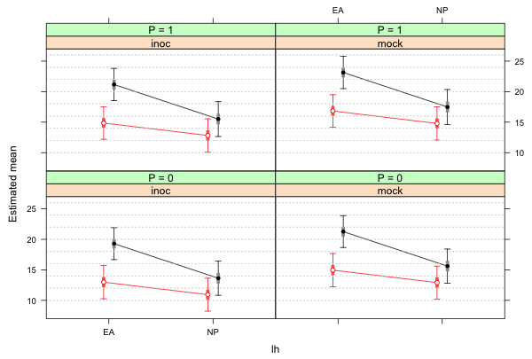Fig. 1   Two-factor interaction panel graph produced by lattice

Adding a key

The use of the key argument was explained in lecture 7. I redo the previous graph but this time add a legend.

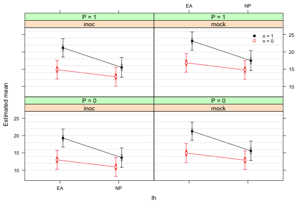Fig. 2   Two-factor interaction panel graph with a legend

Improving the display with the latticeExtra package

The latticeExtra package adds some additional features to the lattice package. One of those features is to allow panel strips on both the sides and tops of the panels. This is possible when the conditioning variable is written as a sum of two factors as it is here. Lattice graphs can be saved as objects that can then be manipulated with functions from latticeExtra. The useOuterStrips function from the latticeExtra package will put panel strips on the left and on the top of the graph.

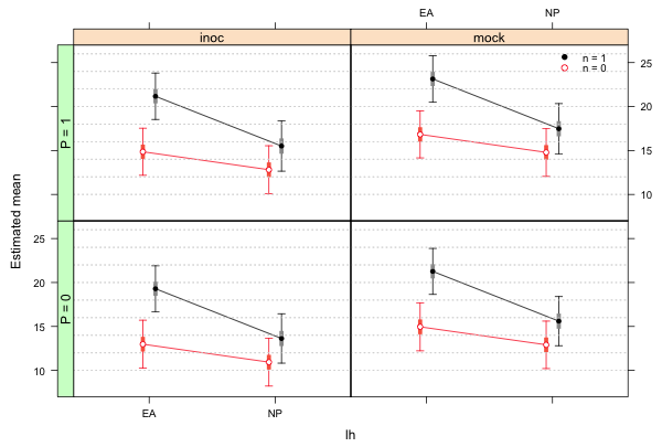Fig. 3   Lattice graph modified by the useOuterStrips function of the latticeExtra package

R Code

A compact collection of all the R code displayed in this document appears here.

Course Home Page