Up until now we’ve worked only with completely randomized statistical designs. In a completely randomized design treatments are randomly assigned to units and the only recognizable differences between those units are the different treatments that have been applied to them. If the units are in fact heterogeneous then the hope is that the random assignment of treatments to units has mixed things up so that on balance the heterogeneity of units assigned to the different treatment groups will be roughly the same.
This is not always optimal. Sometimes we can recognize the heterogeneity of the units ahead of time and wish to take advantage of it. For instance, if we can group similar units together such that each of the similar units gets a different treatment, we could restrict ourselves to making comparisons between the similar units and thus remove some of the background variation that might otherwise make detecting a treatment effect more difficult. If the units are similar then the differences we detect are more likely due to treatment differences. A common example of this is to use genetically related individuals as experimental subjects in which individuals from the same litter or cuttings from the same plant are assigned different treatments. In statistics we use the term block to refer to a group of similar experimental units.
Sometimes the creation of blocks is accidental. The set-up of the experiment may cause some units to be more similar to each other than to others.
In all of these examples the variable that identifies the similar units is called a block. When we include a blocking variable in an analysis we are trying to account for all the things we failed to measure that makes one block different from the next block (and make the individuals in the same block more similar to each other). Statistically a block appears in a regression model as just another categorical variable. So, it would seem that a block is no different than an ordinary factor in analysis of variance. This is more or less true but there are some fundamental differences in how we treat blocks and treatments in regression models.
This example comes from Sokal and Rohlf (1995), p. 365. "Blakeslee (1921) studied length/width ratios of second seedling leaves of two types of Jimsonweed called globe (G) and nominal (N). Three seeds of each type were planted in 16 pots. Is there sufficient evidence to conclude that globe and nominal differ in length/width ratio?" The file jimsonweed.txt is a tab-delimited text file.
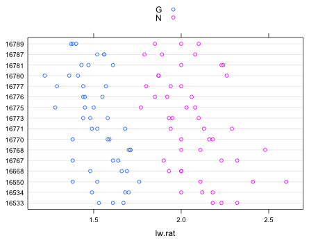
We can examine the structure of the data set by using a dot plot in which we display the length-width ratios of plants from different pots using different colors to denote the different treatments. For this I use the dotplot function from lattice. To color observations by the levels of the treatment variable "type" I specify that variable in the groups argument of dotplot. To get a crude key that identifies the groups I include the argument auto.key=T.
| |
| Fig. 1 Dot plot of length-width ratios separately by pot colored by treatment |
Even if we didn't know that this was a randomized block design the blocking structure is immediately apparent from Fig. 1. In a completely randomized design with treatments randomly assigned to plants and pot playing no role in the treatment assignment we would not be seeing an equal number of G and N treatment assignments in each pot. It's also obvious from Fig. 1 that there is a marked treatment effect with nominal (N) plants having a larger length-width ratio than globe (G) plants. This pattern holds up in every pot which suggests that there is no interaction between treatment and block.
Fig. 1 does reveal some systematic differences across pots (whole distributions are shifted to the left or the right) so accounting for the blocking in the analysis is potentially useful. One unusual thing about this experiment is that treatments are replicated within blocks (pots). Thus we will be able to formally test for a block × treatment interaction.
Because a block is just a categorical variable we can use analysis of variance type models to analyze the randomized block design. Below I fit an additive model (pot + type) and an interaction model (pot*type) to the data. Because the variable that labels the pot categories is numeric I have to convert it explicitly to a factor in the function call.
Response: lw.rat
Df Sum Sq Mean Sq F value Pr(>F)
factor(pot) 15 0.8977 0.0598 3.373 0.000342 ***
type 1 7.3206 7.3206 412.575 < 2.2e-16 ***
factor(pot):type 15 0.3050 0.0203 1.146 0.336418
Residuals 64 1.1356 0.0177
---
Signif. codes: 0 ‘***’ 0.001 ‘**’ 0.01 ‘*’ 0.05 ‘.’ 0.1 ‘ ’ 1
From the ANOVA table we see that block × treatment interaction is not significant. On the other hand both the treatment and block effects are statistically significant.
Response: lw.rat
Df Sum Sq Mean Sq F value Pr(>F)
factor(pot) 15 0.8977 0.0598 3.282 0.0002944 ***
type 1 7.3206 7.3206 401.444 < 2.2e-16 ***
Residuals 79 1.4406 0.0182
---
Signif. codes: 0 ‘***’ 0.001 ‘**’ 0.01 ‘*’ 0.05 ‘.’ 0.1 ‘ ’ 1
It's worthwhile at this point to compare the randomized block design results with what we would have obtained had we ignored the blocking structure of the experiment and had instead carried out a one-way analysis of variance (which in this example is just an independent samples t-test).
Response: lw.rat
Df Sum Sq Mean Sq F value Pr(>F)
type 1 7.3206 7.3206 294.28 < 2.2e-16 ***
Residuals 94 2.3384 0.0249
---
Signif. codes: 0 ‘***’ 0.001 ‘**’ 0.01 ‘*’ 0.05 ‘.’ 0.1 ‘ ’ 1
The crucial thing to look at in comparing these models is the mean squared error. This is the estimate of the background noise that is then used as the gold standard in the construction of the reported F-tests. For the randomized block design the mean squared error is reported to be 0.0182; for the one-way analysis of variance it is 0.0249. So there's about a 25% reduction in the variance that has been accounted for by the blocking.
If we examine the summary table of the model we see that we've estimated a large number of uninteresting terms, the block effects.
Residuals:
Min 1Q Median 3Q Max
-0.30719 -0.09349 0.01333 0.08010 0.36052
Coefficients:
Estimate Std. Error t value Pr(>|t|)
(Intercept) 1.64719 0.05683 28.986 < 2e-16 ***
factor(pot)16534 -0.06167 0.07797 -0.791 0.43134
factor(pot)16550 0.04000 0.07797 0.513 0.60935
factor(pot)16668 -0.13000 0.07797 -1.667 0.09939 .
factor(pot)16767 -0.07667 0.07797 -0.983 0.32844
factor(pot)16768 0.02833 0.07797 0.363 0.71727
factor(pot)16770 -0.10833 0.07797 -1.390 0.16858
factor(pot)16771 -0.08167 0.07797 -1.047 0.29807
factor(pot)16773 -0.17667 0.07797 -2.266 0.02619 *
factor(pot)16775 -0.23833 0.07797 -3.057 0.00305 **
factor(pot)16776 -0.21167 0.07797 -2.715 0.00814 **
factor(pot)16777 -0.25000 0.07797 -3.207 0.00194 **
factor(pot)16780 -0.25833 0.07797 -3.313 0.00139 **
factor(pot)16781 -0.09333 0.07797 -1.197 0.23484
factor(pot)16787 -0.19000 0.07797 -2.437 0.01706 *
factor(pot)16789 -0.24000 0.07797 -3.078 0.00286 **
typeN 0.55229 0.02756 20.036 < 2e-16 ***
---
Signif. codes: 0 ‘***’ 0.001 ‘**’ 0.01 ‘*’ 0.05 ‘.’ 0.1 ‘ ’ 1
Residual standard error: 0.135 on 79 degrees of freedom
Multiple R-squared: 0.8509, Adjusted R-squared: 0.8206
F-statistic: 28.17 on 16 and 79 DF, p-value: < 2.2e-16
The only interesting estimate, the treatment effect, appears at the bottom. From the output we conclude that the mean length-width ratio of nominal (N) plants is 0.553 units bigger than it is for globe (G) plants.
So the above analysis provides an estimate of the treatment effect but if we want to know what the average length-width ratios are for the two treatment groups then we have a problem. If this were a one-way analysis of variance model then the intercept would represent the mean length-width ratio for globe plants and to obtain the mean for nominal plants we would just add the treatment effect 0.552 to the intercept. In a two-way design the intercept represents the mean response when both factors are set to their reference values. Similarly in a randomized block design the intercept represents the mean response when the treatment is at its reference value and block is at its reference value. So, in the above design the intercept, 1.647, is the mean length-ratio for a globe plant that was reared in pot #16533, the reference block. When we add the treatment effect to this value we obtain the mean length-ratio for a nominal plant but again only for those plants reared in pot #16533.
So, in order to obtain the length-width ratio for a given treatment we have to specify a pot number too. If we try to use the predict function on the model just specifying values for type, R complains that it doesn't have enough information.
If instead we create a data frame consisting of values of type and pot in all possible combinations we can obtain the treatment means for the specific pots used in the experiment.
So while the randomized design when analyzed in the fashion described above is useful for estimating treatment effects it is not particularly useful for estimating treatment means.
The analysis we carried out above is called the fixed effects approach to the randomized complete block design (RCBD). In it we define separate sets of dummy variables for treatment and block. If i denotes the block, here numbered 1 through 16, and j the observation in that block, j = 1 through 6, then we create the following set of dummy variables.
 ,
, 
The model for the mean response is
and the model for an individual observation is
where ![]() . In this formulation the intercept β0 represents the mean response for type = 'G' in block 1, β1 is the treatment effect which is the same in each block (because there is no interaction), and β2 through β16 are individual block effects.
. In this formulation the intercept β0 represents the mean response for type = 'G' in block 1, β1 is the treatment effect which is the same in each block (because there is no interaction), and β2 through β16 are individual block effects.
There is a second way to formulate the RCBD using what are called random effects. In this approach the model for the mean is the following.
![]()
and the model for an individual observation is
|
|
(1) |
|---|
where as before ![]() but in addition
but in addition ![]() . The u0i are called random effects, more specifically in the RCBD, random intercepts. There is one random effect for each block, a total of 16 in all for the current design. They are called random effects because they have a distribution instead of being constants like the βi parameters in the model. The βi are called fixed effects, the u0i are called random effects, and the entire model is called a mixed effects model.
. The u0i are called random effects, more specifically in the RCBD, random intercepts. There is one random effect for each block, a total of 16 in all for the current design. They are called random effects because they have a distribution instead of being constants like the βi parameters in the model. The βi are called fixed effects, the u0i are called random effects, and the entire model is called a mixed effects model.
According to the distributional assumption the random effects have a mean of zero, as do the random errors. Thus if we take the mean of eqn (1) we obtain just the fixed effects portion of the model: ![]() . So in the mixed effects approach, unlike the fixed effects model of the RCBD, the fixed effects portion of the model corresponds to the treatment mean averaged over all the blocks. β0 is the mean length-width ratio for the globe plants averaged across pots and β0 + β1 is the mean length-width ratio for the nominal plants averaged across pots. If the blocks used in the experiment are a random sample from a population of such blocks then it is legitimate to refer to the fixed effect portion of the model as the population-average model.
. So in the mixed effects approach, unlike the fixed effects model of the RCBD, the fixed effects portion of the model corresponds to the treatment mean averaged over all the blocks. β0 is the mean length-width ratio for the globe plants averaged across pots and β0 + β1 is the mean length-width ratio for the nominal plants averaged across pots. If the blocks used in the experiment are a random sample from a population of such blocks then it is legitimate to refer to the fixed effect portion of the model as the population-average model.
For an ordinary linear regression model least squares provides us with an explicit solution for the regression parameters. For a mixed effects model there is no explicit solution; parameter estimates have to be obtained iteratively using some variation of Newton's method. Two different packages in R can be used to fit mixed effects models: nlme and lme4. The nlme package is the older of the two and can only fit models in which the response variable has a normal distribution. It is best suited for fitting models with what are called hierarchical random effects. We previously used the gls function from the nlme package in lecture 3. The lme4 package is a recent development and extends the nlme package to include additional probability distributions for the response besides the normal distribution. It can also fit models with both crossed and hierarchical random effects. I illustrate fitting the RCBD to the jimsonweed data using both packages.
Although the nlme package is part of the standard installation of R, it still needs to be loaded into memory at the start of each R session. The function in the nlme package that fits linear regression models with random effects is called lme, for linear mixed effects models. Its syntax is the same as lm except for an additional random argument in which the random effects specification is described.
Notice the syntax that appears in the random argument: ~1|pot.
The anova function when applied to an lme object produces a fairly standard ANOVA table. The blocks don't appear in the table because they are part of random effects formulation of the model.
The summary table for the model provides an estimate of the intercept β0, the treatment effect β1, the standard deviation of the error distribution, σ, and the standard deviation of the random effects distribution, τ.
Random effects:
Formula: ~1 | pot
(Intercept) Residual
StdDev: 0.08328042 0.1350398
Fixed effects: lw.rat ~ type
Value Std.Error DF t-value p-value
(Intercept) 1.5191667 0.02851996 79 53.26679 0
typeN 0.5522917 0.02756488 79 20.03607 0
Correlation:
(Intr)
typeN -0.483
Standardized Within-Group Residuals:
Min Q1 Med Q3 Max
-1.89568380 -0.65943997 0.02981137 0.62150485 3.04884738
Number of Observations: 96
Number of Groups: 16
I've highlighted the entries in the summary table corresponding to the parameter estimates.
To extract the two regression coefficients β0 and β1 from the model object we can use the fixef function.
If we use the coef function, which serves this purpose for lm objects, we get a very different kind of output.
Notice that we get 16 pairs of estimators for β0 and β1, one for each of the 16 blocks (pots). The value for β1 is the same for each but the value of the intercept varies by block. What's being returned here are the random intercepts defined by
![]()
These consist of the overall population intercept plus a prediction of the individual block random effects. To see the predictions of the random effects alone use the ranef function.
These random effects are not obtained as part of the ordinary estimation protocol that returns estimates of β0, β1, σ, and τ, but instead are obtained afterwards using these estimates. For that reason they are usually called predictions rather than estimates. They are variously called empirical Bayes predictions (estimates) or BLUPs (best linear unbiased predictors).
The predict function works with lme objects. If you apply the predict function to an lme model object you obtain the predicted means for each observation used to fit the model. There are 96 observations in the data set so below I just display the predictions for the first twelve.
Notice that the predicted mean changes when we switch blocks. By default the predict function returns an estimate for the mean that includes the block effects. Thus it returns ![]() for globe plants and
for globe plants and ![]() for nominal plants. To obtain predictions of the mean that don't include the random effects we have to specify the level argument of predict (an argument that is only appropriate for lme objects) and set it to level=0.
for nominal plants. To obtain predictions of the mean that don't include the random effects we have to specify the level argument of predict (an argument that is only appropriate for lme objects) and set it to level=0.
Now we see that the globe and nominal means are the same for plants coming from different blocks.
The lme4 package is not part of the standard R installation so it must be downloaded first from the CRAN site. Because the lme4 package is still undergoing active development you'll probably want to make sure you have the latest version of R too. When you load lme4 into memory with the library function you'll obtain some warning messages about objects being masked.
The following object(s) are masked from ‘package:nlme’:
lmList, VarCorr
The following object(s) are masked from ‘package:stats’:
AIC, BIC
Some of the functions in the lme4 and nlme packages have the same name. To ensure that the correct function is called when you need it you should unload the nlme package from memory by using the detach function.
The function in the lme4 package that fits linear mixed effects models is lmer. The lmer function does not have a random argument. Instead the random effects specification is included as part of the regression model as follows.
Notice that in the lme function we specified: random=~1|pot. Here we include (1|pot) as a term in the model. Both the anova and summary functions work on lmer objects.
Fixed effects:
Estimate Std. Error t value
(Intercept) 1.51917 0.02852 53.27
typeN 0.55229 0.02756 20.04
Correlation of Fixed Effects:
(Intr)
typeN -0.483
If you compare the estimates reported by lmer with those reported by lme, they are the same. One noticeable difference between the lme output and the lmer output is that lmer reports the values of test statistics, but it does not report p-values.
The absence of p-values in the output from lmer is by design. The author of the lme4 package, Douglas Bates, argues that there is no legitimate method using standard probability distributions for obtaining p-values for the F- and t-statistics of mixed effects models that will work in all cases. His explanation can be found here and is summarized briefly below.
There are problems with the approach used by nlme.
There have been lots of recommendations for obtaining correct p-values of test statistics in mixed effects models but none of these apply in general. For example, SAS offers the user a number of different ways to carry out tests and calculate p-values but leaves it up to the user to choose one. Some of these approaches are clearly good choices for a few special cases, e.g., balanced data with a simple structure, but none of these are general solutions.
We can make the following general recommendations for carrying out hypothesis testing in mixed effects models (Faraway 2010).
The parametric bootstrap is a Monte Carlo method for obtaining the empirical distribution of a test statistic of interest. In this method we fit a model of interest to a sequence of simulated data sets where the simulation is carried out in such a way that the null hypothesis is true. For each simulation we calculate the test statistic whose distribution we don't know. The set of test statistics we obtain estimates the null distribution of our test statistic. We then determine the position of the actual test statistic, the one that was calculated using the real data, in this null distribution. If it is an extreme value in this distribution we have reason to reject the null hypothesis. Formally we can obtain a p-value for the test by counting up the number of simulated test statistics as large or larger than the actual test statistic (for a one-tailed test) and divide this by the total number of simulations. Usually the actual test statistic is counted as one of the simulations so the number of simulated test statistics as large as or larger than the actual test statistic is always at least one.
We can use the parametric bootstrap to obtain a p-value for the F-statistic for the variable type that is reported by the anova function when applied to an lmer object. The F-statistic lies in row 1, column 4 of the anova output.
Next we fit a mixed effects model to the plants data set but we don't include type as a predictor. The model includes only the random intercepts.
We now use this model to generate new data sets. Data sets generated from this model will have the same random effects structure as do our actual data. By construction the variable type will not be a predictor of the response (because the response variable was generated without it). We fit a mixed effects model to each simulated data set in which we include type as a predictor. Because the simulated response does not depend on type the F-statistics we obtain from these fits provide a null distribution for the F-statistic for type.
In the code below I carry out 999 simulations each time extracting the F-statistic. I initialize a vector using the numeric function to store the results of the simulations. I use a for loop to perform the iterations and the simulate function to generate data from the lmer model. In the end I append the actual F-statistic as one additional simulation to yield a total of 1000.
The largest simulated F-statistic is 9.42 while the actual F-statistic exceeds 400. Since the actual F-statistic is the largest of the simulated F-statistics our p-value is 1 out of 1000, or .001. The F-test of type is statistically significant.
We will discuss Bayesian estimation in greater detail later in this course, so at this point I give only a cursory introduction. The standard statistical methods we've covered so far in this course are called frequentist methods. The logical foundation of the frequentist approach is based on the notion of a sampling distribution. Parameters are thought to be fixed in a nature, but a statistic that is used to estimate that parameter being based on a sample varies. If we were to obtain a different sample of the same size from the same population the value of the statistic would probably be different. The set of statistics calculated from all possible samples from the population yields the sampling distribution of the statistic. The sampling distribution is the basis for constructing confidence intervals and carrying out statistical tests in the frequentist approach.
The Bayesian school of statistics approaches statistical estimation from a different philosophical viewpoint. Bayesians are indifferent to the notion of whether there exists a true value of a parameter in nature. From a Bayesian point of view what we know about a parameter is really just a matter of opinion. Being rational beings we should formulate our opinions as probability statements that quantify what are the likely values of the parameter. Before we collect any data we generally have some opinion about what values the parameter might take. This is called our prior distribution for the parameter. If we truly don't know anything about the parameter then we have what's called a flat or uninformative prior. After collecting data or carrying out an experiment we use the information contained in the data to update our prior opinion about the parameter. Our updated opinion is called the posterior distribution of the parameter.
The modern way of carrying out Bayesian estimation is via Markov chain Monte Carlo (MCMC) sampling. MCMC doesn't provide formulas for the posterior distributions of parameters, instead it yields samples from these distributions. Using these samples we can then calculate summary statistics to characterize the distributions of the parameters. For instance we could calculate means or medians of the distribution and use them as point estimates. For interval estimates we can calculate the .025 and .975 quantiles of the sampled posterior distributions to obtain 95% confidence intervals for the parameters (although Bayesians prefer to use the term credible intervals).
R provides the mcmcsamp function as a simple way to obtain Bayesian parameter estimates using a frequentist model fit with lmer. To use mcmcsamp we supply the name of the lmer model plus the number of desired samples from the posterior distribution. There are a number of diagnostics that one should look at to verify that the Markov chain has stabilized and is truly sampling from the posterior distribution. We'll ignore those issues for now and explore them at a later date when we formally consider Bayesian estimation. In the call below I use the lmer model mod2.lmer and request 10,000 samples.
To organize the output from mcmcsamp in the form of a data frame we can use the as.data.frame function.
The data frame contains samples from the posterior distribution of the intercept β0, the treatment effect β1 labeled "typeN", the standard deviation of the errors "sigma", and ST1 which is the ratio of the random effects standard deviation to the error standard deviation, τ/σ. To obtain point estimates of these parameters we can take the mean or median of each of the columns of the data frame. These values compare favorably with the point estimates returned by lmer.
To obtain 95% confidence (credible) intervals for the parameters we can extract the .025 and .975 quantiles of each column with the quantile function.
Because the 95% credible interval for the treatment effect (typeN) does not include zero we can conclude that the length-width ratios of globe and nominal jimsonweed plants are significantly different. Bayesians generally prefer to calculate something called an HPD (highest probability density) interval instead of a percentile interval. The HPD intervals can be obtained by applying the HPDinterval function directly to the original mcmcsamp object. In the output below the differences between the HPD intervals and the percentile intervals obtained above are fairly small.
$ST
lower upper
[1,] 0.163902 0.7560056
attr(,"Probability")
[1] 0.95
$sigma
lower upper
[1,] 0.1196254 0.1654788
attr(,"Probability")
[1] 0.95
What's especially attractive about Bayesian estimation is that we can easily obtain interval estimates for functions of parameter estimates. In the mixed effects model β0 is the mean length-width ratio of the globe plants while β0 + β1 is the mean length-width ratio of nominal plants. To obtain a sample from the posterior distribution of the mean length-width ratio of nominal plants we just add the sample from the posterior distribution of β0 to the sample from the posterior distribution of β1. Intervals estimates for the treatment means can be obtained by calculating quantiles of the posterior distributions.
Because the 95% credible intervals don't overlap we can say that the mean length-width ratios of the two plant types are significantly different.
A compact collection of all the R code displayed in this document appears here.
| Jack Weiss Phone: (919) 962-5930 E-Mail: jack_weiss@unc.edu Address: Curriculum for the Environment and Ecology, Box 3275, University of North Carolina, Chapel Hill, 27599 Copyright © 2012 Last Revised--September 17, 2012 URL: https://sakai.unc.edu/access/content/group/3d1eb92e-7848-4f55-90c3-7c72a54e7e43/public/docs/lectures/lecture6.htm |