Last time we considered a randomized block design. The experiment we examined had multiple plants growing in the same pot as well as plants growing in different plots for a total of 96 plants organized in 16 pots. The six plants per pot consisted of two types: three plants of type 'G' and three plants of type 'N'. If we think of type as a treatment that was randomly applied to individual plants then this design is an example of restricted randomization. Among the six plants in any pot three were always assigned to one treatment and three to the other treatment. Notice that this is not the same as randomly assigning 48 plants to one treatment and 48 plants to the other and then randomly dividing them among the 16 pots.
Last time we considered two different ways to analyze these data. The first was as a fixed effects model in which block was treated as a factor and the analysis resembled a two-factor analysis of variance. Because the treatments are replicated within blocks we were able to test for a block × treatment interaction. We found that the interaction was not significant so we dropped it. The final model was additive in blocks and treatments.
Response: lw.rat
Df Sum Sq Mean Sq F value Pr(>F)
factor(pot) 15 0.8977 0.0598 3.373 0.000342 ***
type 1 7.3206 7.3206 412.575 < 2.2e-16 ***
factor(pot):type 15 0.3050 0.0203 1.146 0.336418
Residuals 64 1.1356 0.0177
---
Signif. codes: 0 ‘***’ 0.001 ‘**’ 0.01 ‘*’ 0.05 ‘.’ 0.1 ‘ ’ 1
Although the randomized block design looks like a two-way analysis of variance there are some subtle differences. For instance, most statistics texts would argue that a formal test for block effects in a randomized block design is not appropriate. Typically in the RCBD we can't test for a block × treatment interaction because there is no replication of treatments within blocks. What would normally constitute the interaction sum of squares is instead used as the error term in testing for a treatment effect. But the ratio of the mean squares for blocks to the mean squares for interaction does not have an F-distribution and so there is no valid test for blocks in this case. This problem is not an issue with the current design because we have replication of treatments within blocks.
The second argument against testing for a block effect is that unlike the treatments, blocks are usually not randomly assigned to subjects. (Again, that is technically not the case here where plants could have been randomly assigned to pots.) Some authors attempt to formalize this further by defining an additional error variance that they call restriction error that is peculiar to block designs. The absence of randomization of subjects to blocks technically makes the F-test for blocks invalid.
The basic point is that blocks are philosophically different from treatments. They are part of the design structure rather than the treatment structure. As a result we should retain them regardless of what we discover about them after the fact. If it turns out they didn't make much of a difference there's nothing we can do about it. We deliberately altered our experimental design to include them. We chose a restricted randomization in which treatments were randomly assigned within individual blocks, not across blocks. Dropping blocks from the analysis at this point would be to claim that we had actually carried out a completely randomized design, which is not true. The loss in degrees of freedom in the MSE that we suffer due to blocking is the penalty we pay for a bad design choice.
Two complications that arise with the fixed effects approach to a randomized block design is that (1) we end up with estimates of block effects that we don't care about and (2) when we try to predict the mean response for individual treatments we get the treatment means for a specific block (the reference block) rather than for an average block. We can get around both of these difficulties by treating blocks as a random effect rather than a fixed effect. When block effects are treated as random effects we view the treatments as defining the population mean structure about which individual blocks deviate randomly. In fitting this model we formally estimate the parameters of the probability distribution of the blocks rather than the individual block effects.
One way of fitting a model in which block effects are treated as random is with the nlme package.
To extract the fixed estimates of the intercept and the treatment effect we use fixef. To extract predictions of the random effects we use ranef. To obtain estimates of the intercepts that vary by block we use coef. The predict function can be used to obtain estimates of the population means for individual observations. The predict function by itself returns the estimated mean for each observation in the data set using both the fixed effects and random effects. These are sometimes called the conditional means. To obtain only the fixed effects prediction of the mean requires using the level=0 argument of predict. These are called the marginal means, or, if the data can be treated as a random sample from a known population, the population average means. The newdata argument of predict can be used with lme objects to predict the means of new observations. The fitted function when applied to an lme object also returns estimates of the conditional means.
Last time we didn't discuss how to obtain confidence intervals of the parameter estimates returned by lme. One way to calculate them is by extracting parameter estimates and their standard errors and then selecting the appropriate t-distribution or normal distribution multiplier to use in the standard confidence interval formula. A second way for obtaining confidence intervals is to use the intervals function of the nlme package.
Fixed effects:
lower est. upper
(Intercept) 1.4623991 1.5191667 1.5759342
typeN 0.4974252 0.5522917 0.6071582
attr(,"label")
[1] "Fixed effects:"
Random Effects:
Level: pot
lower est. upper
sd((Intercept)) 0.04955372 0.08328042 0.1399618
Within-group standard error:
lower est. upper
0.1155431 0.1350398 0.1578263
By default the intervals function returns confidence intervals for the fixed effect parameters as well as the standard deviations of the normal distributions of the errors and random effects. To obtain only the confidence intervals for the fixed effect parameters we can use the which='fixed' argument of intervals.
Fixed effects:
lower est. upper
(Intercept) 1.4623991 1.5191667 1.5759342
typeN 0.4974252 0.5522917 0.6071582
attr(,"label")
[1] "Fixed effects:"
A second way of fitting a model in which the block effects are treated as random is with the lme4 package. The syntax is a bit different from nlme.
The fixef, ranef, and coef functions work the same way as with lme. Unlike lme there is no predict method for mer objects.
The methods function of R can be used to determine if a particular package has supplied a method for a given function. The output below shows the available methods for predict from all the packages installed in my version of R. Notice that there are methods for nlme, lme, and gls objects (all created by the nlme package), but none listed for lmer.
The fitted function does work with the output from lmer and from lme. It returns predicted means for each observation in the data frame using both the fixed and random effects.
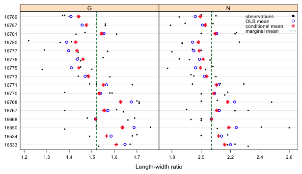
For the randomized block design that we've been considering, there are three kinds of means we can obtain for individual observations. One type is the ordinary least squares mean obtained by fitting an lm model in which both treatments and blocks are treated as fixed effects. Two additional means from a mixed effects model are the marginal and conditional means. It might be worthwhile to compare these different means in a single diagram in which we superimpose the means on a plot of the raw data.
I begin by collecting the OLS and conditional means in a data frame and then adding them to the data frame of the raw data. For the mixed effects model I use the output from lmer.
To calculate the marginal means from the lmer object I just use the regression formula. The intercept, coef(mod2.lmer)[1], is the mean for type = 'G'. The intercept plus the treatment effect, coef(mod2.lmer)[1] + coef(mod2.lmer)[2], is the mean for type = 'N'. To add this mean to the data frame I use the ifelse function. The first argument of ifelse is a logical condition, the second argument is the value to return if the condition evaluates to TRUE, and the third argument is the value to return if the condition evaluates to FALSE.
The ifelse function works with vectors component-wise so for each observation we can test if type == 'G' and have ifelse return the appropriate mean based on the result of evaluating the test condition.
I display the length-width ratios using a dot plot. For this I use two new panel functions: panel.points and panel.grid. The panel.points function is the lattice analog of the points function of base graphics and adds points to a graph. The panel.grid function adds grid lines. I specify v=0 to prevent vertical grid lines from being displayed and h=-16 to get 16 horizontal grid lines to display at the 16 tick marks.
| |
| Fig. 1 Dot plot of length-width ratios for each pot separately by treatment. The raw data, OLS means (blocks treated as fixed effects), conditional means (which include predictions of the block random effects), and marginal means (averages over all blocks) are shown. |
The main new feature in this code is the use of subscripts in the list of arguments of the panel function. When the panel function is called upon to draw a panel the variable subscripts indicates the value of type (the variable that defines the panels) that is being used for the current panel. It takes the form of a Boolean vector of TRUEs and FALSEs. So, in the above code the expressions new.dat3$fix.ests[subscripts] and new.dat3$mix.est[subscripts] extract a vector of OLS means and a vector of conditional means corresponding to the level of type that is currently being plotted. This is the same role the arguments x and y have in the function. By default each time a panel is drawn the correct set of pot and lw.rat values (the x and y variables) are selected. Because fix.ests and mix.est were not part of the original function call we have to extract the correct set of observations for them explicitly.
I use the scales argument with value list(x='free') to specify that the x-limits can be different in the two panels.
The jitter function adds random noise to the y-coordinate of the observed points, by default, up to 20% of the closest distance between points in the y-direction. This allows us to distinguish observations in the same block that have the same length-width ratios. The jitter amount can be specified explicitly with the amount argument of jitter. The jitter function requires a numeric argument so I have to first convert the factor to its numeric value with as.numeric(y).
The key argument is mostly self-explanatory. The key itself is an R object called a list that is here created with the list function. A list object in R is one whose components can be of various types and of different lengths.
Notice that in all cases in Fig. 1 the conditional mean is located between the marginal mean (vertical line) and the OLS mean. We say that the conditional means are shrunk towards the population mean. The shrinkage occurs because the random effects are constrained to come from a common distribution and are not totally free to vary as the OLS means are. If we had an unequal number of observations in the groups, the estimates for groups with more observations would typically be shrunk less than the estimates for groups with fewer observations. Because of shrinkage mixed effects models are less affected by anomalous data values and are less prone overfitting the data.
As was explained last time it is more typical in randomized block designs to not have any replication of treatments within blocks. To illustrate a situation where this occurs I consider a data set in the faraway package that is meant to supplement Faraway (2005). The data set is called oatvar and can be loaded with the data function.
Faraway (2005) describes the data as follows, p. 204. "We illustrate this with an experiment to compare eight varieties of oats. The growing area was heterogeneous and so was grouped into five blocks. Each variety was sown once within each block and the yield in grams per 16-ft row was recorded. The data come from Anderson and Bancroft (1952)." If we tabulate the data by block and variety we see that there is one observation per treatment within each block.
The lack of replication means that we can't fit a model in which block and treatment interact. If we try to fit this model the anova function issues a warning and the ANOVA table does not report any F-statistics or p-values. The summary table for the coefficients has missing values for standard errors and test statistics (not shown).
Response: yield
Df Sum Sq Mean Sq F value Pr(>F)
block 4 33396 8348.9
variety 7 77524 11074.8
block:variety 28 37433 1336.9
Residuals 0 0
Warning message:
In anova.lm(g1) :
ANOVA F-tests on an essentially perfect fit are unreliable
On the other hand there is no problem in fitting a model that is additive in block and treatment. Controlling for blocks we find that there is a significant effect of variety.
Response: yield
Df Sum Sq Mean Sq F value Pr(>F)
block 4 33396 8348.9 6.2449 0.001008 **
variety 7 77524 11074.8 8.2839 1.804e-05 ***
Residuals 28 37433 1336.9
---
Signif. codes: 0 ‘***’ 0.001 ‘**’ 0.01 ‘*’ 0.05 ‘.’ 0.1 ‘ ’ 1
The randomized block design with interaction can be written generically as follows.
![]()
Here αi denotes the effect of block i and βj denotes the effect of treatment j. Without replication we can't formally test for interaction and we have to assume (αβ)ij = 0 for all i and j. While we can't test for a generic interaction it is possible to test for specific forms of the interaction. One test of this kind is the Tukey test for non-additivity. To use the test we have to assume that the interaction can be written as a product of the block and treatment effects.
![]()
We can fit this model by estimating the additive model, extracting the coefficient estimates for αi and βj, constructing the product term using these estimates, and refitting the model with this term to test if the coefficient of the product term is significantly different from zero.
The block estimates are in positions 2 through 5 and the treatment estimates are in positions 6 through 12. The first block effect and the first treatment effect are both zero (because we are using reference cell coding for the effects), so I prepend a zero to the block and treatment vectors.
To match the layout in the oatvar data frame each element of the treatment vector needs to be repeated five times (once for each block) while the entire block effect vector needs to be repeated eight times. To make the arrangement clear I assemble everything in a data frame and display the first few observations.
I add the multiplicative term to the additive model and carry out a significance test.
Response: yield
Df Sum Sq Mean Sq F value Pr(>F)
block 4 33396 8348.9 6.0563 0.001299 **
variety 7 77524 11074.8 8.0337 2.787e-05 ***
ab 1 213 212.9 0.1544 0.697428
Residuals 27 37220 1378.5
---
Signif. codes: 0 ‘***’ 0.001 ‘**’ 0.01 ‘*’ 0.05 ‘.’ 0.1 ‘ ’ 1
The multiplicative term is not significant thus we can reject the presence of an interaction of the form posited by the Tukey test.
Graphical methods of assessing interaction are applicable here. For instance we can produce a dot plot of yield by block in which we identify the different treatments by symbol type and color. Adding the groups argument to a lattice plot function causes the points to be plotted with different colors. To get different symbols too I specify the pch argument with eight different values.
To get a legend we could create our own using the key argument as was done in Fig. 1. Alternatively we can use the auto.key argument. For auto.key to work we have to reset the global pch setting for groups for lattice graphs to 1:8. Lattice works differently from base graphics. The graphical parameter setting for groups is contained in the components of the superpose.symbol parameter. We can obtain the current settings of this lattice graphics parameter with trellis.par.get.
$cex
[1] 0.8 0.8 0.8 0.8 0.8 0.8 0.8
$col
[1] "#0080ff" "#ff00ff" "darkgreen" "#ff0000" "orange" "#00ff00" "brown"
$fill
[1] "#CCFFFF" "#FFCCFF" "#CCFFCC" "#FFE5CC" "#CCE6FF" "#FFFFCC" "#FFCCCC"
$font
[1] 1 1 1 1 1 1 1
$pch
[1] 1 1 1 1 1 1 1
Notice that the default symbol type is 1 for all groups. To change the settings we need to use the trellis.par.set function. The following call changes the settings for pch to 1:8.
$cex
[1] 0.8 0.8 0.8 0.8 0.8 0.8 0.8
$col
[1] "#0080ff" "#ff00ff" "darkgreen" "#ff0000" "orange" "#00ff00" "brown"
$fill
[1] "#CCFFFF" "#FFCCFF" "#CCFFCC" "#FFE5CC" "#CCE6FF" "#FFFFCC" "#FFCCCC"
$font
[1] 1 1 1 1 1 1 1
$pch
[1] 1 2 3 4 5 6 7 8
Now we can use the auto.key argument and specify that the legend should appear on the right side of the graph with the space argument.
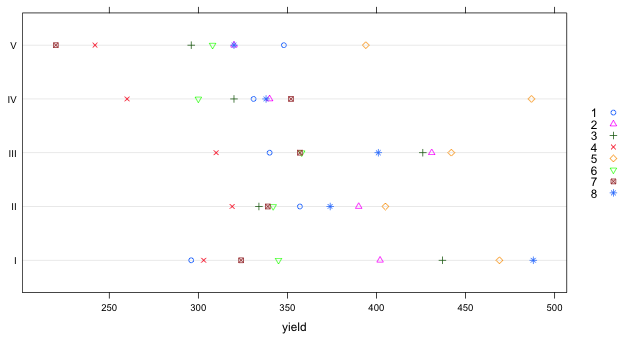 |
| Fig. 2 Dot plot of yields separately by block with individual treatments indicated |
Notice that the ranking of treatments (by yield) is more or less consistent across blocks. For instance, treatment 4 yields either the lowest yield (in three blocks) or the second lowest yield (in two blocks). Similarly treatment 5 yields the highest yield in four of the five blocks, and the second highest yield in one block. There are some inconsistencies across blocks. For instance treatment 7 ranks worst in block V but in the other four blocks it is never worse than third worst.
Alternatively we can generate a crude interaction plot with the interaction.plot function of R. The first argument of interaction.plot defines the variable to plot on the x-axis, the second argument is the variable that defines the profiles, and the last variable defines what is to be plotted. In Fig. 3 I plot yield against variety separately for each block.
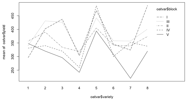 |
| Fig. 3 Interaction plot showing the variability of treatment effects by block |
In Fig. 3 we need to determine if the block profiles are parallel. Notice that if we look only at varieties 3, 4, 5, and 6 the parallel assumption seem reasonable. If we look at varieties 1 and 2 or varieties 7 and 8 the rankings of the treatments within blocks appear to change. What we can say is that the deviations from additivity that we can detect in Fig. 3 are not especially dramatic.
Blocking can be part of any experimental design. We next consider an experiment in which the treatments consist of combining the levels of four factors (each with two levels) in all possible ways.
The factors comprising the treatment are lh (a life history trait), func (an indicator of whether the plant was infected with virus), and nutrient treatments n and p. The response is pN, the percent nitrogen composition of the plant. If we tabulate the treatments we see that the data are unbalanced with between 6 and 12 observations per treatment.
inoc mock
EA 7 7
NP 9 9
, , = 1, = 0
inoc mock
EA 12 12
NP 7 7
, , = 0, = 1
inoc mock
EA 10 10
NP 8 8
, , = 1, = 1
inoc mock
EA 10 10
NP 6 6
In addition to the treatment structure there is a blocking variable (five blocks) and a variable phy that indicates the type of grass plant. It turns out that not every treatment appeared in every block. To see this I create a treatment variable by concatenating the levels of the four factor variables with the paste function of R. The paste function has a sep argument that permits a separator to be placed between each of the character values. I use a period to serve as the separator between the factor levels.
I tabulate the treatment variable against block and against phy.
We can see that there are a lot of zeros so not every treatment is represented in every block. Blocks 3, 4, and 6 have missing treatments. The situation for the three grass types is similar. Only "TRI" is represented in all 16 treatments.
The researcher chose to fit models in which the square of pN was the response, a very strange choice. He also chose to drop the observation corresponding to tag #444. I fit his basic model that included block and phy as well as a 4-factor interaction between lh, func, n and p. I then consider Type I and Type II tests of all the terms in the model that are related to treatment.
Response: pN^2
Df Sum Sq Mean Sq F value Pr(>F)
factor(block) 5 264.59 52.92 4.1968 0.0015441 **
factor(phy) 2 229.04 114.52 9.0822 0.0002188 ***
factor(lh) 1 739.16 739.16 58.6214 6.749e-12 ***
factor(n) 1 634.83 634.83 50.3471 1.165e-10 ***
factor(func) 1 135.19 135.19 10.7217 0.0014025 **
factor(p) 1 101.81 101.81 8.0744 0.0053200 **
factor(lh):factor(n) 1 105.33 105.33 8.3534 0.0046098 **
factor(lh):factor(func) 1 24.33 24.33 1.9292 0.1675527
factor(n):factor(func) 1 8.48 8.48 0.6723 0.4139756
factor(lh):factor(p) 1 5.52 5.52 0.4375 0.5096631
factor(n):factor(p) 1 26.63 26.63 2.1122 0.1488793
factor(func):factor(p) 1 1.09 1.09 0.0865 0.7692047
factor(lh):factor(n):factor(func) 1 28.18 28.18 2.2350 0.1376806
factor(lh):factor(n):factor(p) 1 15.94 15.94 1.2638 0.2632881
factor(lh):factor(func):factor(p) 1 36.27 36.27 2.8762 0.0926295 .
factor(n):factor(func):factor(p) 1 13.75 13.75 1.0903 0.2986082
factor(lh):factor(n):factor(func):factor(p) 1 1.96 1.96 0.1555 0.6940604
Residuals 114 1437.43 12.61
---
Signif. codes: 0 ‘***’ 0.001 ‘**’ 0.01 ‘*’ 0.05 ‘.’ 0.1 ‘ ’ 1
Response: pN^2
Sum Sq Df F value Pr(>F)
factor(block) 288.20 5 4.5713 0.0007754 ***
factor(phy) 208.54 2 8.2694 0.0004430 ***
factor(lh) 446.58 1 35.4177 2.995e-08 ***
factor(n) 687.74 1 54.5433 2.698e-11 ***
factor(func) 134.25 1 10.6474 0.0014549 **
factor(p) 109.82 1 8.7095 0.0038434 **
factor(lh):factor(n) 101.30 1 8.0339 0.0054320 **
factor(lh):factor(func) 24.92 1 1.9760 0.1625351
factor(n):factor(func) 6.14 1 0.4871 0.4866400
factor(lh):factor(p) 2.71 1 0.2146 0.6440844
factor(n):factor(p) 26.66 1 2.1144 0.1486659
factor(func):factor(p) 0.61 1 0.0486 0.8258384
factor(lh):factor(n):factor(func) 21.77 1 1.7269 0.1914517
factor(lh):factor(n):factor(p) 15.75 1 1.2493 0.2660352
factor(lh):factor(func):factor(p) 41.59 1 3.2981 0.0719899 .
factor(n):factor(func):factor(p) 13.75 1 1.0903 0.2986082
factor(lh):factor(n):factor(func):factor(p) 1.96 1 0.1555 0.6940604
Residuals 1437.43 114
---
Signif. codes: 0 ‘***’ 0.001 ‘**’ 0.01 ‘*’ 0.05 ‘.’ 0.1 ‘ ’ 1
It's clear from the output that the 4-factor interaction can be dropped. From the Type II tests we see that none of the 3-factor interactions are significant when added last, although the lh:func:p interaction comes close. Although the Type I tests add the 3-factor interactions in a different order they also agree with the the Type II tests. Still we might want to consider a model in which lh:func:p is the first 3-factor interaction added.
From the Type I tests the lh:n interaction appears to be significant. The Type II tests are in agreement with this. We should realize that the Type II tests of the two-factor interactions are rather strange here because the reference model includes some of the three-factor interactions too. For instance, the Anova function tests the term factor(func):factor(n) by fitting a model that contains all main effects, all two-factor interactions, and any higher order interaction that doesn’t also contain the term factor(func):factor(n). It then compares this to the same model in which the term factor(func):factor(n) has been dropped. The reference model then is one with all two-factor interactions and main effects plus the two three-factor interactions factor(func):factor(lh):factor(p) and factor(lh):factor(n):factor(p).
I next fit a model with all two-factor interactions and try adding back in the lh:func:p three-factor interaction.
Response: pN^2
Df Sum Sq Mean Sq F value Pr(>F)
factor(block) 5 264.59 52.92 4.1841 0.0015504 **
factor(phy) 2 229.04 114.52 9.0548 0.0002196 ***
factor(lh) 1 739.16 739.16 58.4449 6.153e-12 ***
factor(n) 1 634.83 634.83 50.1955 1.090e-10 ***
factor(func) 1 135.19 135.19 10.6894 0.0014123 **
factor(p) 1 101.81 101.81 8.0501 0.0053576 **
factor(lh):factor(n) 1 105.33 105.33 8.3283 0.0046425 **
factor(lh):factor(func) 1 24.33 24.33 1.9234 0.1680970
factor(lh):factor(p) 1 5.44 5.44 0.4299 0.5133070
factor(n):factor(func) 1 8.56 8.56 0.6765 0.4124502
factor(n):factor(p) 1 26.63 26.63 2.1058 0.1493942
factor(func):factor(p) 1 1.09 1.09 0.0862 0.7695245
factor(lh):factor(func):factor(p) 1 41.16 41.16 3.2545 0.0737780 .
Residuals 118 1492.36 12.65
---
Signif. codes: 0 ‘***’ 0.001 ‘**’ 0.01 ‘*’ 0.05 ‘.’ 0.1 ‘ ’ 1
So, we don't need to include any of the three-factor interactions. I next consider the Type II tests for the model that contains all two-factor interactions.
Response: pN^2
Sum Sq Df F value Pr(>F)
factor(block) 280.80 5 4.3579 0.0011186 **
factor(phy) 223.94 2 8.6886 0.0003005 ***
factor(lh) 444.88 1 34.5224 3.922e-08 ***
factor(n) 689.40 1 53.4967 3.284e-11 ***
factor(func) 133.67 1 10.3724 0.0016496 **
factor(p) 109.19 1 8.4731 0.0043039 **
factor(lh):factor(n) 100.83 1 7.8246 0.0060126 **
factor(lh):factor(func) 26.51 1 2.0570 0.1541314
factor(lh):factor(p) 2.86 1 0.2220 0.6383522
factor(n):factor(func) 8.12 1 0.6300 0.4289362
factor(n):factor(p) 26.57 1 2.0618 0.1536520
factor(func):factor(p) 1.09 1 0.0846 0.7716120
Residuals 1533.52 119
---
Signif. codes: 0 ‘***’ 0.001 ‘**’ 0.01 ‘*’ 0.05 ‘.’ 0.1 ‘ ’ 1
The Type II and Type I tests combined suggest that only the lh × n interaction needs to be retained. I fit that model and examine the remaining terms.
Response: pN^2
Df Sum Sq Mean Sq F value Pr(>F)
factor(block) 5 264.59 52.92 4.1022 0.0017588 **
factor(phy) 2 229.04 114.52 8.8775 0.0002493 ***
factor(lh) 1 739.16 739.16 57.3005 7.391e-12 ***
factor(n) 1 634.83 634.83 49.2127 1.317e-10 ***
factor(func) 1 135.19 135.19 10.4801 0.0015481 **
factor(p) 1 101.81 101.81 7.8924 0.0057698 **
factor(lh):factor(n) 1 105.33 105.33 8.1652 0.0050096 **
Residuals 124 1599.56 12.90
---
Signif. codes: 0 ‘***’ 0.001 ‘**’ 0.01 ‘*’ 0.05 ‘.’ 0.1 ‘ ’ 1
Response: pN^2
Sum Sq Df F value Pr(>F)
factor(block) 294.16 5 4.5607 0.0007486 ***
factor(phy) 217.45 2 8.4284 0.0003698 ***
factor(lh) 427.11 1 33.1098 6.426e-08 ***
factor(n) 686.40 1 53.2103 3.117e-11 ***
factor(func) 134.70 1 10.4417 0.0015780 **
factor(p) 108.85 1 8.4378 0.0043527 **
factor(lh):factor(n) 105.33 1 8.1652 0.0050096 **
Residuals 1599.56 124
---
Signif. codes: 0 ‘***’ 0.001 ‘**’ 0.01 ‘*’ 0.05 ‘.’ 0.1 ‘ ’ 1
Based on the output we have a significant interaction between lh and n as well as significant main effects for func and p.
As we've previously seen, treating block as a fixed effect allows us to estimate treatment differences, but it makes obtaining sensible treatment means more difficult. To get around this I treat block as a random effect and refit the final model above with random blocks rather than fixed blocks.
The F-statistics in the ANOVA table of the mixed effects model are nearly identical to the F-statistics from the ANOVA table of Type I tests for the fixed effects block model.
Depending upon how we view the variable phy we might also choose to make phy random. If the species used were of no special interest and were merely selected to be representative of a larger pool of possible species then we might be more interested in the average treatment mean for a typical plant (irrespective of species) than the mean of a plant of a specific species. This would also be a good approach if we had predictors that grouped species in various ways that might explain any differences between the species. Of course with only three species, as is the case here, treating species as random might be a bit suspect.
The species and block variables are crossed (rather than nested) in this design, i.e., they are found in all possible combinations. A cross random effects model for observation k of species j from block i can be written as follows.
![]()
![]()
The term μijk is short hand notation for the fixed effect part of the model that arises from the treatment structure. The lme4 package is well-suited for estimating models with crossed random effects. We just need to include two random terms in the model.
The ANOVA table is nearly the same as what we obtained with lme and only random blocks. If we examine the summary table we see that the variability between species exceeds the variability between blocks.
Fixed effects:
Estimate Std. Error t value
(Intercept) 12.9810 1.3909 9.333
factor(lh)NP -2.0468 0.9416 -2.174
factor(n)1 6.3092 0.8492 7.430
factor(func)mock 1.9742 0.6132 3.219
factor(p)1 1.8754 0.6302 2.976
factor(lh)NP:factor(n)1 -3.6139 1.2702 -2.845
Correlation of Fixed Effects:
(Intr) fc()NP fctr(n)1 fctr() fctr(p)1
factr(lh)NP -0.347
factor(n)1 -0.372 0.565
fctr(fnc)mc -0.221 -0.013 -0.001
factor(p)1 -0.269 0.086 0.105 0.006
fct()NP:()1 0.241 -0.691 -0.659 0.008 -0.038
A compact collection of all the R code displayed in this document appears here.
| Jack Weiss Phone: (919) 962-5930 E-Mail: jack_weiss@unc.edu Address: Curriculum for the Environment and Ecology, Box 3275, University of North Carolina, Chapel Hill, 27599 Copyright © 2012 Last Revised--September 25, 2012 URL: https://sakai.unc.edu/access/content/group/3d1eb92e-7848-4f55-90c3-7c72a54e7e43/public/docs/lectures/lecture7.htm |