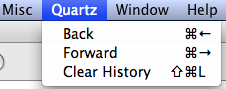
Fig. 1 (a) Menu selection in Windows OS to stack multiple graphs and pages of graphs in the same window. (b) Menu selection in Mac OS X to move "Back" to previous pages of graphs produced in a Quartz window.
Last time we created a lattice graph with 29 panels. This approaches the practical limit on the number of panels that can be reasonably displayed on a single page. We can spread a panel graph across multiple pages by specifying a value for the layout argument that corresponds to a subset of the panels. The code below recreates the goodness of fit panel graph from last time but specifies that only 16 panels should be displayed on the same page.
When a multi-page graph is created in R only the last page of the multi-page graph will be displayed in the graphics window. In Windows OS the graphics window has a History menu option. If the Recording option of History menu had previously been checked (Fig. 1a) each graph is stored as a separate page of the graphics window. Pressing the PgUp or PgDown keys on the keyboard allows you to navigate to different pages in the graphics window. Note: For this to work the Recording option must be selected before you create the graph. In Mac OS X the Quartz menu has the options Back and Forward (with the keyboard shortcuts shown in Fig. 1b) for navigating to previous pages of a multi-page graph.
| (a) |
(b) |
Fig. 1 (a) Menu selection in Windows OS to stack multiple graphs and pages of graphs in the same window. (b) Menu selection in Mac OS X to move "Back" to previous pages of graphs produced in a Quartz window. |
|
It's also possible to pause the graph before each page is displayed by specifying par(ask=T) at the R prompt. R displays the message "Hit <Return> to see next plot:" Pressing the <enter> key causes the next page of the graph to be displayed. Continue pressing <enter> until all pages are displayed. To disable this option enter par(ask=F).
I refit the Poisson model for the species-area relationship. Highlighted in the output from the summary function below is a statistic called the residual deviance.
Deviance Residuals:
Min 1Q Median 3Q Max
-10.4912 -3.6827 -0.9111 2.0992 10.0887
Coefficients:
Estimate Std. Error z value Pr(>|z|)
(Intercept) 3.240970 0.043050 75.28 <2e-16 ***
log(Area) 0.342991 0.007346 46.69 <2e-16 ***
---
Signif. codes: 0 ‘***’ 0.001 ‘**’ 0.01 ‘*’ 0.05 ‘.’ 0.1 ‘ ’ 1
(Dispersion parameter for poisson family taken to be 1)
Null deviance: 3447.59 on 28 degrees of freedom
Residual deviance: 640.22 on 27 degrees of freedom
AIC: 800.03
Number of Fisher Scoring iterations: 5
Historically a quantity called the deviance has played an important role in assessing the fit of a Poisson regression model, although in truth it's only sometimes appropriate. The deviance is reported in the summary table of the Poisson model where it is called the residual deviance. The deviance can be derived from the usual likelihood ratio statistic as follows.
Suppose we have two nested models with estimated parameter sets ![]() and
and ![]() and corresponding likelihoods
and corresponding likelihoods ![]() and
and ![]() . If
. If ![]() is a special case of
is a special case of ![]() then we can compare the models using a likelihood ratio test.
then we can compare the models using a likelihood ratio test.
Recall that LR has an asymptotic chi-squared distribution with degrees of freedom equal to the difference in the number of parameters estimated by the two models. Alternatively, the degrees of freedom is the number of parameters that are fixed to have a specific value in one model but are freely estimated in the other model.
Now suppose the model with likelihood ![]() is the saturated model. A saturated model is one in which one parameter is estimated for each observation. For a saturated Poisson model λi = yi, i.e., the Poisson mean for each observation is the observed count. A likelihood ratio statistic that compares the current model with a saturated model is the residual deviance of that model. We can demonstrate this by calculating the likelihood ratio statistic by hand.
is the saturated model. A saturated model is one in which one parameter is estimated for each observation. For a saturated Poisson model λi = yi, i.e., the Poisson mean for each observation is the observed count. A likelihood ratio statistic that compares the current model with a saturated model is the residual deviance of that model. We can demonstrate this by calculating the likelihood ratio statistic by hand.
For the saturated model there are n parameters, one for each observation. The likelihood ratio statistic has an asymptotic chi-squared distribution with degrees of freedom equal to the difference in the number of estimated parameters of the two nested models. I calculate this difference by hand.
Notice that 27 is exactly what is reported as the degrees of freedom for the residual deviance in the summary table. The saturated model fits the data perfectly, i.e., it fits it as well as a Poisson model can. If our model is not significantly different from the saturated model we conclude that our model fits as well as a perfect model. Given that our model does so with fewer parameters we should prefer our model because it is more parsimonious.
If we carry out the residual deviance test here we obtain a significant result. Assuming that the test is valid we conclude that our model is significantly different from the saturated model and hence that we have a significant lack of fit.
The probability mass function for a Poisson random variable is
If ![]() is the maximum likelihood estimate of λ for observation i, i = 1, … , n, then the log-likelihood of a Poisson regression model with n observations is the following.
is the maximum likelihood estimate of λ for observation i, i = 1, … , n, then the log-likelihood of a Poisson regression model with n observations is the following.
For the saturated model the maximum likelihood estimate of λ is yi and the corresponding log-likelihood is the following.
Subtracting these quantities and doubling the difference yields the residual deviance for the Poisson model.
Define
then
![]()
is called a deviance residual. Here sign denotes the sign function which is defined as follows.
The deviance residual measures the ith observation's contribution to the deviance. Since under ideal conditions the deviance can be used as a measure of lack of fit, the deviance residual measures the ith observation's contribution to model lack of fit. If we square the deviance residuals and sum them we obtain the residual deviance. We can extract the deviance residuals from a Poisson regression model with the residuals function by specifying type = 'deviance'.
The chi-squared distribution of the likelihood ratio test is an asymptotic result. The likelihood ratio statistic has a chi-squared distribution only as the sample size gets large. Implicit in this statement is that the sample size should get large while the difference in the number of estimated parameters in the two models remains fixed. This is not the case when one of the models is the saturated model because as the sample size gets large, so does the number of parameters (because there is one parameter per observation). This can invalidate the assumed chi-squared distribution of the residual deviance.
It turns out that the residual deviance for a Poisson regression model is equal to the G-statistic (in the notation of Sokal and Rohlf, 1995). The G test, often called the likelihood ratio chi-squared test, is an alternative to the Pearson chi-squared test to which it is asymptotically equivalent. The G-test is defined as follows.
If we calculate this statistic for the current model we see that we obtain the residual deviance.
Like the Pearson chi-squared statistic, the G-statistic has an asymptotic chi-squared distribution with n – p degrees of freedom where p is the number of estimated parameters. Also like the Pearson statistic the validity of the chi-squared distribution of the G-statistic depends on some minimal sample size restrictions on the counts. If none of the expected counts are less than 1 and no more than 20% are less than 5, then the chi-squared distribution is reasonable. If we check this condition here we find that all of the expected counts exceed 5.
Therefore the goodness of fit test based on the residual deviance is probably valid for these data and we can conclude that the Poisson regression model does not adequately fit the data.
If we use the formula for the Pearson goodness of fit statistic on the individual observations of the Poisson regression model we obtain what's called the Pearson deviance.
The Pearson deviance is generally considered superior to the residual deviance as a goodness of fit statistic for Poisson regression models (if the minimal sample size criteria are met). It is also compared to a chi-squared distribution with n – p degrees of freedom where p is the number of estimated parameters and n is the sample size. Typically there is little substantive difference between using the residual deviance and the Pearson deviance as a goodness of fit statistic.
The individual terms of the Pearson statistic are called the Pearson residuals, which for a Poisson regression model are the following.

The Pearson residual when squared can be viewed as the contribution the ith observation makes to the Pearson statistic. Because the mean and variance of the Poisson distribution are equal each Pearson residual has the form of a z-score. The Pearson residuals from a glm object can be extracted with the residuals function by specifying type='pearson'. If we square the Pearson residuals and sum them we get the Pearson deviance.
I need to comment on an often spurious seat of the pants rule about the residual deviance that has appeared in the literature and is perpetuated in textbooks and articles about statistics written for ecologists. The rule requires that we calculate the ratio of the residual deviance to its degrees of freedom.
If φ > 1 we say the data are overdispersed relative to a Poisson distribution. If φ < 1 we say the data are underdispersed relative to a Poisson distribution. For the current data set and model we find
so we would say using the fitted model that the data are overdispersed relative to a Poisson distribution meaning that the data show more variability than is predicted by a Poisson distribution.
Technically speaking it's not the deviance based on the G-statistic that is usually used for assessing over- or underdispersion, but instead it is the "deviance" based on the Pearson goodness of fit statistic. If we calculate the ratio of the Pearson deviance to its degrees of freedom we obtain the following.
Once again φ > 1 so we would say the data are overdispersed relative to a Poisson distribution.
The logic behind this rule is that the mean of a chi-squared distribution is equal to its degrees of freedom. So the ratio compares a chi-squared statistic to its mean. But as we noted above, for the residual deviance to have a chi-squared distribution requires that the individual expected counts are all sufficiently large (at most no more than 20% are smaller than 5). So the seat of the pants rule is inappropriate if there are a large number of small expected counts.
Suppose we wish to compare two nested models with likelihoods L1 and L2 where L2 is the "larger" (more estimated parameters) of the two likelihoods. Let LS denote the likelihood of the saturated model. The likelihood ratio statistic for comparing these two models is the following.
where D1 and D2 are the deviances of models 1 and 2, respectively. Thus to carry out a likelihood ratio test to compare two models we can equivalently just compute the differences in their deviances. Because of the parallel to analysis of variance (ANOVA) in ordinary linear models, carrying out an LR test using the deviances of the models is often called analysis of deviance. When we apply the anova function to a glm model the table that is reported is labeled "analysis of deviance" but as we've seen the individual tests that are reported are just the likelihood ratio tests comparing the sequentially nested models.
Model: poisson, link: log
Response: Species
Terms added sequentially (first to last)
Df Deviance Resid. Df Resid. Dev Pr(>Chi)
NULL 28 3447.6
log(Area) 1 2807.4 27 640.2 < 2.2e-16 ***
---
Signif. codes: 0 ‘***’ 0.001 ‘**’ 0.01 ‘*’ 0.05 ‘.’ 0.1 ‘ ’ 1
As counterintuitive as it may seem, it is possible to use Poisson and negative binomial regression to fit models in which the response variable is a rate, the number of events that occur per unit time or per unit area, even when the denominator of the rate is different for different observations. To illustrate how this can be done we consider a data set in which counts of bird species were obtained on various sized tracts of land all over the island of Jamaica. We load the data set and examine the available variables.
The variable S records the bird species richness in a patch in a given year. Each patch was visited up to three times in three consecutive years: 2005 through 2007. The area of each patch was recorded and each patch was assigned a landscape category type of which there are four. The objective was to determine how aluminum mining on the island (landscape = "Bauxite") was affecting bird populations. So we have repeated measures data in which an important covariate, area, was recorded that may modify the nature of the relationship between richness and landscape type. Previously for normally-distributed response variables we used analysis of covariance to adjust for a covariate such as area (lecture 9) and we used a mixed effects (random intercepts) model to account for the repeated measures (lecture 11). The exact same approaches will work when the response variable has a Poisson distribution.
An examination of the gross distribution of bird richness values reveals nothing unusual.
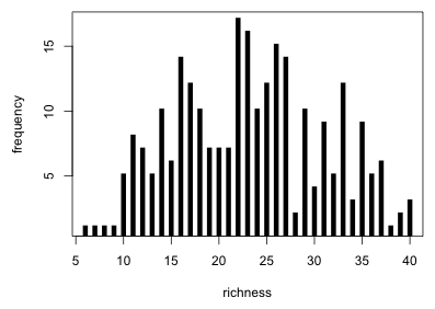 |
Fig. 2 Gross distribution of bird richness values |
Based on what we see either a Poisson or a normal distribution might be a suitable probability model. Keep in mind that Fig. 2 should not necessarily remind us of any distribution in particular. The goal is to model the mean richness using landscape, year, and perhaps other predictors and it's only after the set of observations has been carved up into various subsets by predictors that the choice of probability distribution becomes relevant. For instance, if all the individual subsets are normally distributed it doesn't follow that the overall distribution will also be normally distributed. What we do learn from Fig. 2 is that the distribution is shifted away from zero, so we probably don't have to worry about a normal distribution for richness yielding negative predictions. Furthermore we see that the overall distribution is roughly symmetric so a negative binomial model is probably unnecessary nor will we need to log-transform richness.
I examine the mean bird richness values by landscape and year. Because there are a number of missing values in the response variable I include the additional argument na.rm=T to remove those values. (The tapply function allows additional arguments to the function, in this case mean, to be listed after the function.)
There appear to be important differences in bird richness across the different landscapes. Richness is lowest in urban areas and around bauxite mines. Forested and agricultural areas have much higher richness values. These patterns maintain themselves across all three years but in year 2005 all four landscapes experienced much higher richness values than in subsequent years. These observations suggest that a simple additive model in landscape and year might suffice, the classic main effects two-factor analysis of variance model. Because we're dealing with count data I assume a Poisson distribution for the response with a log link for the mean. With only three years of data it probably makes sense to treat year as a factor.
Model: poisson, link: log
Response: S
Terms added sequentially (first to last)
Df Deviance Resid. Df Resid. Dev P(>|Chi|)
NULL 256 691.67
landscape 3 138.918 253 552.75 < 2.2e-16 ***
factor(year) 2 20.495 251 532.25 3.545e-05 ***
---
Signif. codes: 0 ‘***’ 0.001 ‘**’ 0.01 ‘*’ 0.05 ‘.’ 0.1 ‘ ’ 1
The analysis of deviance table indicates that both landscape and year are significant predictors. I examine the summary table of the model.
Deviance Residuals:
Min 1Q Median 3Q Max
-3.80085 -1.06031 0.05366 0.98796 2.96943
Coefficients:
Estimate Std. Error z value Pr(>|z|)
(Intercept) 3.41323 0.02835 120.416 < 2e-16 ***
landscapeBauxite -0.33365 0.03633 -9.183 < 2e-16 ***
landscapeForest -0.12738 0.03401 -3.745 0.000180 ***
landscapeUrban -0.35814 0.03858 -9.284 < 2e-16 ***
factor(year)2006 -0.13397 0.03317 -4.039 5.36e-05 ***
factor(year)2007 -0.10764 0.03005 -3.581 0.000342 ***
---
Signif. codes: 0 ‘***’ 0.001 ‘**’ 0.01 ‘*’ 0.05 ‘.’ 0.1 ‘ ’ 1
(Dispersion parameter for poisson family taken to be 1)
Null deviance: 691.67 on 256 degrees of freedom
Residual deviance: 532.25 on 251 degrees of freedom
(49 observations deleted due to missingness)
AIC: 1811.3
Number of Fisher Scoring iterations: 4
The summary table confirms the pattern we observed in the gross summary statistics. Agricultural areas have the highest bird richness followed by forested areas. Urban and bauxite areas bring up the rear and are essentially tied. We also see that richness in 2005 was significantly higher than in the two subsequent years.
We're not done yet because we haven't checked fit. It's unwise to draw inferences from a model that doesn't fit the data. The Poisson distribution is one for which the residual deviance can potentially be used as a goodness of fit statistic. I check to see if most of the observations have predicted cell counts that are larger than five.
100% of the expected cell counts are greater than five so the residual deviance can be used a goodness of fit statistic. I examine the ratio of the residual deviance to its degrees of freedom.
The data are overdispersed relative to a Poisson distribution and based on the p-value of the chi-squared test, significantly so. This should not be surprising. The smallest predicted Poisson mean is 18.6 yet in Fig. 2 we saw counts as low as six. Even assuming that these low counts correspond to the patch with the smallest mean, probabilities of obtaining counts this small are extremely low using this Poisson model. This indicates that it is very unlikely that the current model could have generated these data.
An obvious plot characteristic that we'd expect to have a big impact on bird richness is the size of the patch. It turns out the patches vary quite a bit with respect to size.
So, there's a 100-fold difference in plot size in these data. If we examine the mean patch area by landscape type we see marked differences there also.
Agricultural patches were on average more than twice the size of any of the other patch types. Given that our goal to relate richness to landscape, area is an obvious confounding variable. So, we should replace analysis of variance with analysis of covariance treating area or log(area) as a covariate. A plot of richness versus area and richness versus log(area) suggests that log-transforming area yields a better linear relationship with species richness.
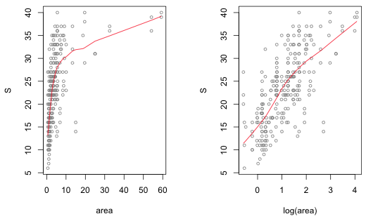 |
Fig. 3 Checking the linear relationship between species richness (S) and area. |
Because we're using a log link for the mean, using log(area) will also yield a more interpretable model. If we use log-likelihood and AIC to compare a model that includes area to a model that uses log(area) as a predictor, the log(area) model has the larger log-likelihood and the smaller AIC.
Deviance Residuals:
Min 1Q Median 3Q Max
-3.79706 -0.75487 0.04366 0.74034 2.24672
Coefficients:
Estimate Std. Error z value Pr(>|z|)
(Intercept) 3.08891 0.03662 84.348 < 2e-16 ***
landscapeBauxite -0.22688 0.03728 -6.086 1.16e-09 ***
landscapeForest -0.06504 0.03441 -1.890 0.058744 .
landscapeUrban -0.27087 0.03931 -6.890 5.57e-12 ***
factor(year)2006 -0.11130 0.03321 -3.351 0.000805 ***
factor(year)2007 -0.10660 0.03005 -3.547 0.000389 ***
log(area) 0.21003 0.01353 15.518 < 2e-16 ***
---
Signif. codes: 0 ‘***’ 0.001 ‘**’ 0.01 ‘*’ 0.05 ‘.’ 0.1 ‘ ’ 1
(Dispersion parameter for poisson family taken to be 1)
Null deviance: 691.67 on 256 degrees of freedom
Residual deviance: 297.53 on 250 degrees of freedom
(49 observations deleted due to missingness)
AIC: 1578.6
Number of Fisher Scoring iterations: 4
The predictor log(area) is highly significant. So, having controlled for differences in area we find that the richness in forested areas is no longer significantly different from the richness in agricultural areas. Apparently the difference we observed in the previous model and in the raw data was due to the much larger size of agricultural patches.
The final model we've obtained has a simple theoretical basis. The fitted model for mean richness in agricultural areas in 2005 is the following.
This is the classic species-area model in which richness is proportional to a power of area. The area exponent is 0.21 so we see that richness scales by the fifth root of area. The role that landscape and year play in this model is to modify the multiplier k but not the basic species-area relationship.
Has adding log(area) to the regression model solved the lack of fit problem? I check again that the expected counts still meet the minimum cell size criterion.
100% of the expected cell counts are still larger than 5, so the residual deviance can be used as a measure of fit. The smallest expected mean count has decreased somewhat but probably not enough to account for some of the smallest counts in the data set.
So, the data are still overdispersed but now only barely so. The chi-squared distribution for the residual deviance indicates that the overdispersion is still statistically significant. So, we may still have a fit problem. This is not surprising because we've been ignoring an important feature of these data, the fact that the same patch is contributing multiple observations to the data set. If a given patch has individual characteristics that cause it to deviate systematically from other patches with the same covariate pattern, that could account for the small amount of overdispersion that remains. We'll consider this possibility below.
When I submitted the above analysis (with a further adjustment for the repeated measures structure that we'll discuss below) to the researcher, she was not satisfied. She explained that she didn't want to model richness; she wanted to model density, the number of species per unit area. Density is generally a difficult quantity to model statistically. Density is a ratio and ratios can be extremely unstable particularly when both the numerator and denominator are measured with error. We can expect to see both very small and very large ratios in the same data set. A further complication is that density is a positive quantity, further constraining our choice of probability models. We previously discussed some of the problems with analyzing ratios in lecture 9.
There are a number of reasons why count observations in a data set might not be equivalent.
In each of these cases it would be more natural to work with the rate of occurrence: the number of observations per unit time, per unit area, or the per capita rate. It is possible to analyze a rate while fitting a Poisson model to the counts if you treat the log of the denominator of the rate as an offset. An offset is the name we use for a regressor whose coefficient is not estimated.
An offset is typically a term of the form, ![]() ,
, ![]() , or
, or ![]() that is included in the model with its coefficient constrained to be equal to 1.
that is included in the model with its coefficient constrained to be equal to 1.
To understand what using an offset is supposed to accomplish consider the Jamaican birds example where the counts are obtained from patches with different sized areas. Suppose that our model has p additional regressors, ![]() . We fit a count regression model for the mean (either as a Poisson or negative binomial regression) using a log link and an offset of
. We fit a count regression model for the mean (either as a Poisson or negative binomial regression) using a log link and an offset of ![]() .
.
![]()
![]() is an offset because it's not multiplied by a parameter. Its coefficient is 1, although any numeric multiplier could in principle be used. An equivalent way to write this equation is the following.
is an offset because it's not multiplied by a parameter. Its coefficient is 1, although any numeric multiplier could in principle be used. An equivalent way to write this equation is the following.
Thus by including an offset we end up fitting a model for the rate of occurrence, counts per unit area, as was desired. The use of an offset then is just a trick that allows us to use Poisson or negative binomial regression, methods that are appropriate for count data, to fit a rate model.
The glm function has an offset argument for specifying the variable to use as an offset. For regression functions without an offset argument, such as lm and glm.nb, offsets can still be included in a regression model by using the offset function.
The following is completely equivalent.
If we examine the summary table we see that the offset doesn't appear anywhere except in the listed formula. Because the coefficient of log(area) is not estimated, no coefficient is reported in the summary table.
Deviance Residuals:
Min 1Q Median 3Q Max
-13.5597 -0.1101 1.5889 3.3103 9.7338
Coefficients:
Estimate Std. Error z value Pr(>|z|)
(Intercept) 1.19264 0.02786 42.802 < 2e-16 ***
landscapeBauxite 0.57236 0.03672 15.586 < 2e-16 ***
landscapeForest 0.55630 0.03401 16.355 < 2e-16 ***
landscapeUrban 0.57255 0.03903 14.668 < 2e-16 ***
factor(year)2006 0.02139 0.03351 0.639 0.523
factor(year)2007 -0.11795 0.03001 -3.930 8.49e-05 ***
---
Signif. codes: 0 ‘***’ 0.001 ‘**’ 0.01 ‘*’ 0.05 ‘.’ 0.1 ‘ ’ 1
(Dispersion parameter for poisson family taken to be 1)
Null deviance: 4250.4 on 256 degrees of freedom
Residual deviance: 3798.6 on 251 degrees of freedom
(49 observations deleted due to missingness)
AIC: 5077.7
Number of Fisher Scoring iterations: 5
When we include log(area) as an offset in a regression model we constrain its regression coefficient to be one. One way to determine if the use of an offset is justified is by fitting the analysis of covariance model and testing whether the regression coefficient of log(area) is equal to 1, i.e., test H0: β = 1. We previously fit the analysis of covariance model so I use the confint function to obtain 95% confidence intervals for the regression parameters.
The 95% confidence interval for the coefficient of log(area) is (0.18, 0.24). Because this interval does not include 1 we can reject a coefficient of 1 as being a reasonable value at the α = .05 level. We can also assess the appropriateness of the offset model with AIC. If we compare the AICs of the various Poisson models we've fit, we see that the Poisson model with a log area offset appears to be a terrible model. The analysis of covariance model ranks best.
The inclusion of an offset in a Poisson regression model is done primarily for purposes of interpretation. If interpreting the response as a rate is not interesting, but controlling for the lack of equivalence of the observations is, it is perfectly legitimate to include time, area, or population size in the model as a covariate. Covariates generally are variables that are of no interest by themselves but are included solely because it is believed that to omit them would have deleterious effects. When a predictor is included as a covariate rather than as an offset, its regression coefficient is estimated instead of being set to one. When a variable is included as a covariate it may not be necessary or desirable to log-transform it first as was done when it was entered as an offset. My personal choice is to always include a potential offset as a covariate rather than as an offset. If it does turn out that the estimated coefficient of the covariate is not significantly different from 1, then and only then might I replace it with an offset and thus save a degree of freedom. I prefer to let the data tell me if treating the response as a density or a rate is the correct choice to make.
We've already noted that the Jamaican birds data set is a repeated measures design with measurements made over three years. Bird counts were obtained from the same patch in multiple years although not every patch was visited every year, so the data are unbalanced.
We see that 12 patches were visited once, 22 patches were visited twice, and 67 patches were visited for all three years. There was no interest in tracking bird richness over time. The concern was that using only a single year of data could be misleading if that year happened to be particularly good or particularly bad for birds. As was discussed in lecture 11 repeated measures designs yield heterogeneous data. Observations from the same patch in different years might be expected to be more similar to each other than they are to observations from different patches in the same or different years.
One way to account for this heterogeneity is to introduce a term that is shared by all observations from the same patch. Because we're not particularly interested in the value of this term we make it a random effect, a parameter whose values are drawn from a probability distribution. This specific kind of mixed effects model is called a random intercepts model. Let i denote the patch and j the observation made on that patch. The model we're fitting is the following.
So, in this model we assume that the population log mean richness in 2005 for patches in agricultural areas with area = 1 are drawn from a common population with mean β0. To obtain the mean in a particular patch we add to β0 the patch-level random effects u0i, which vary from patch to patch. These patch means all then shift by an amount β1 in 2006 and by an amount β2 in year 2007 relative to their values in 2005. The patch mean is further affected by the landscape type and the area of the patch.
The Poisson random intercepts model is fit in R with the lmer function from the the lme4 package as follows.
Fixed effects:
Estimate Std. Error z value Pr(>|z|)
(Intercept) 3.06613 0.05170 59.31 < 2e-16 ***
landscapeBauxite -0.22858 0.05531 -4.13 3.58e-05 ***
landscapeForest -0.06744 0.05205 -1.30 0.195084
landscapeUrban -0.26663 0.05855 -4.55 5.26e-06 ***
factor(year)2006 -0.13039 0.03389 -3.85 0.000119 ***
factor(year)2007 -0.10911 0.03044 -3.58 0.000339 ***
log(area) 0.22222 0.02100 10.58 < 2e-16 ***
---
Signif. codes: 0 ‘***’ 0.001 ‘**’ 0.01 ‘*’ 0.05 ‘.’ 0.1 ‘ ’ 1
From the summary output we see that the between patch variance τ2 is estimated to be 0.019. When we compare the summary table of the random intercept model to the summary table of a model without random effects the changes in the point estimates are rather small.
Deviance Residuals:
Min 1Q Median 3Q Max
-3.7971 -0.7549 0.0437 0.7403 2.2467
Coefficients:
Estimate Std. Error z value Pr(>|z|)
(Intercept) 3.08891 0.03662 84.348 < 2e-16 ***
landscapeBauxite -0.22688 0.03728 -6.086 1.16e-09 ***
landscapeForest -0.06504 0.03441 -1.890 0.058744 .
landscapeUrban -0.27087 0.03931 -6.890 5.57e-12 ***
factor(year)2006 -0.11130 0.03321 -3.351 0.000805 ***
factor(year)2007 -0.10660 0.03005 -3.547 0.000389 ***
log(area) 0.21003 0.01353 15.518 < 2e-16 ***
---
Signif. codes: 0 ‘***’ 0.001 ‘**’ 0.01 ‘*’ 0.05 ‘.’ 0.1 ‘ ’ 1
(Dispersion parameter for poisson family taken to be 1)
Null deviance: 691.67 on 256 degrees of freedom
Residual deviance: 297.53 on 250 degrees of freedom
(49 observations deleted due to missingness)
AIC: 1578.6
Number of Fisher Scoring iterations: 4
More striking though is the fairly large increase in the standard errors of the landscape effects in the random intercepts model. Such an increase should be expected because without the random effects we are treating the individual measurements made on the same patch but in different years as independent replicates of the landscape effect. This is pseudo-replication and by including a random effect that links these measurements together and recognizes their correlation we've obtained a more realistic estimate of the precision of the landscape effect.
It would be nice to be able to use AIC to compare this model to the unstructured Poisson model, but it turns out that the log-likelihood values reported by the lmer function aren't comparable to those generated from other distributions or using other R functions. (The AIC from lmer can be used to compare other Poisson mixed effects models.)
A naive interpretation of the output would suggest that the mixed effects model is a dramatic improvement over the ordinary Poisson regression model, but this isn't necessarily correct. Apparently a portion of the log-likelihood not involving the parameters has been left out of the log-likelihood that is reported by lmer. To correct for this we need to calculate the log-likelihood ourselves. To this end the next section presents some basic information on the likelihood of random effects models.
The switch from a pure fixed effects model to a random intercepts model leads to a fundamental change in the likelihood that is being maximized. Because both the response variable and the random effects have a probability distribution, together they have a joint probability distribution. From our standpoint the random effects are nuisance parameters. The likelihood we desire is the the likelihood of the data without the random effects. We can obtain this likelihood by integrating the joint likelihood with respect to the random effects. The trick in all this is to recognize that a joint probability function can be written as the product of a conditional distribution and a marginal distribution, each of which is a known distribution. It is this product that we then integrate to obtain the desired likelihood.
In much of what follows I use generic notation for the distributions involved because the ideas carry over to other distributions other than the Poisson distribution that we're focused on here. I assume that the observations come in clusters and that the clusters are a random sample from a population of clusters. The clusters for the Jamaican birds example are the patches.
Methods employing maximum likelihood all start with the likelihood function. Recall that if we have a random sample of observations, ![]() , that are independent and identically distributed with probability density (mass) function
, that are independent and identically distributed with probability density (mass) function ![]() where θ is potentially a vector of parameters of interest, then the likelihood of our sample is the product of the individual density functions. For the Poisson regression model θ will consist solely of the set of regression parameters β so that the likelihood can be written as follows.
where θ is potentially a vector of parameters of interest, then the likelihood of our sample is the product of the individual density functions. For the Poisson regression model θ will consist solely of the set of regression parameters β so that the likelihood can be written as follows.
With correlated data, i.e., structured data, the situation is more complicated. The data consist of observations ![]() where i indicates the level-2 unit (cluster) and j the level-1 observation within that unit. Typically the level-2 units will be independent but the level-1 units will not be. If we let
where i indicates the level-2 unit (cluster) and j the level-1 observation within that unit. Typically the level-2 units will be independent but the level-1 units will not be. If we let
![]()
so that ![]() , then we can write the likelihood in terms of the m level-2 units as follows.
, then we can write the likelihood in terms of the m level-2 units as follows.
If we choose to model the hierarchical structure using a mixed effects model then the ![]() are not the only random quantities to consider. The random effects
are not the only random quantities to consider. The random effects ![]() also have a distribution. Thus the natural starting place in constructing the likelihood is with the joint density function of the data and random effect in cluster i,
also have a distribution. Thus the natural starting place in constructing the likelihood is with the joint density function of the data and random effect in cluster i, ![]() . From elementary probability theory we can write
. From elementary probability theory we can write
![]()
Let ![]() . If we include the regression parameters in the likelihood then the joint distribution of the data and the random effects in cluster i would be written as follows
. If we include the regression parameters in the likelihood then the joint distribution of the data and the random effects in cluster i would be written as follows
![]()
Conditional on the value of the random effect, the individual ![]() in cluster i are assumed to be independent. So we have
in cluster i are assumed to be independent. So we have
Here I use ![]() to denote the distribution of the individual
to denote the distribution of the individual ![]() conditional on the random effect and the regression and variance parameters.
conditional on the random effect and the regression and variance parameters.
To go from the joint probability of ![]() and
and ![]() to the marginal probability for
to the marginal probability for ![]() we integrate over the possible values of
we integrate over the possible values of ![]() . Thus the marginal likelihood for cluster i is the following.
. Thus the marginal likelihood for cluster i is the following.
Putting all these pieces together we can write the marginal likelihood of our data as follows.
For the Jamaican birds random intercepts model the distribution of the random effects is normal and the distribution of the response given the random effects is Poisson. Thus the functions k and h in the last expression are a Poisson probability and a normal density respectively.
This expression doesn't simplify further (unlike the case when both k and h are normal densities) and so the integration needs to be carried out numerically in order to obtain the marginal likelihood. This is what the lmer function of the lme4 package does.
To obtain the correct marginal log-likelihood for a Poisson random intercepts model that we can then use to compare with ordinary Poisson regression models I've written a function that inserts the maximum likelihood estimates returned by lmer into the above expression for the joint log-likelihood that I then integrate numerically to obtain the correct marginal log-likelihood. This function is shown below.
To use it here we just provide it with the name of the Poisson random intercepts model that was fit by lmer. There is an additional argument that may be needed to get the integral to converge, but it is not needed for this problem.
If we compare this to the log-likelihood of the ordinary Poisson regression model without random intercepts we see that the log-likelihood of the random effects model is larger.
To compare the AICs we need the number of estimated parameters in the random intercepts model. This should be one more than it is for the ordinary Poisson regression model, the extra parameter being τ2, the variance of the random effects. Alternatively we can extract this information using the attr function applied to the output from logLik.
Comparing the AICs we obtain the following.
So the AIC of the random intercepts model, 1540.97, is appreciably lower than the AIC of the ordinary Poisson regression model. To check the fit of the random intercepts model we would next need to carry out a predictive simulation using the fitted means to generate Poisson distributions like we've done previously for other examples and assess how closely the pseudo-data that are generated resemble the data that were actually obtained.
Sokal, Robert R. and F. J. Rohlf. 1995. Biometry. W. H. Freeman and Company: New York.
A compact collection of all the R code displayed in this document appears here.
| Jack Weiss Phone: (919) 962-5930 E-Mail: jack_weiss@unc.edu Address: Curriculum for the Environment and Ecology, Box 3275, University of North Carolina, Chapel Hill, 27599 Copyright © 2012 Last Revised--November 11, 2012 URL: https://sakai.unc.edu/access/content/group/3d1eb92e-7848-4f55-90c3-7c72a54e7e43/public/docs/lectures/lecture22.htm |