Assignment 5—Solution
Question 1
I save the .csv version of the file to my hard disk and read it into R. I then retain only those observations that have non-missing values for both Brain_Mass and Body_Mass.
mammals <- read.csv('ecol 563/brainbody.csv')
names(mammals)
[1] "Updated_Species_Name" "Species_Name"
[3] "Species_Order" "Brain_Volume"
[5] "Brain_Volume_Standard_Deviation" "Brain_Mass"
[7] "Brain_Mass_Standard_Deviation" "Body_Mass"
[9] "Body_Mass_Standard_Deviation" "Sex"
[11] "No_Individuals" "Age_Class"
[13] "Source" "Notes"
dim(mammals)
[1] 1998 14
mammals2 <- mammals[!is.na(mammals$Brain_Mass) & !is.na(mammals$Body_Mass),]
dim(mammals2)
[1] 1818 14
Question 2
I tabulate the occurrences of the various orders in the data frame.
table(mammals2$Species_Order)
Afrosoricida Carnivora Cetartiodactyla Cetartiodactyla Chiroptera
17 173 164 1 59
Dasyuromorphia Didelphimorphia Diprotodontia Erinaceomorpha Eulipotyphla
51 20 124 19 44
Hyracoidea Lagomorpha Macroscelidea Microbiotheria Notoryctemorphia
5 25 4 1 1
Paucituberculata Peramelemorphia Perissodactyla Primates Proboscidea
2 15 12 622 10
Rodentia Scandentia Sirenia Tubulidentata Xenarthra
409 5 7 1 27
There is a typo in Cetartiodactyla; one individual was recorded with a trailing space. We can fix that in a number of ways.
Method 1: Using ifelse
mammals2$Species_Order <- ifelse(mammals2$Species_Order == 'Cetartiodactyla ', 'Cetartiodactyla', as.character(mammals2$Species_Order))
Method 2: Using grep
grep('Cetartiodactyla ', mammals2$Species_Order)
[1] 1727
mammals2$Species_Order[1727] <- 'Cetartiodactyla'
Method 3: Using sub
mammals2$Species_Order <- sub('Cetartiodactyla ', 'Cetartiodactyla', mammals2$Species_Order)
Method 4: Using trim
library(gdata)
mammals2$Species_Order <- trim(mammals2$Species_Order)
table(mammals2$Species_Order)
Afrosoricida Carnivora Cetartiodactyla Chiroptera Dasyuromorphia
17 173 165 59 51
Didelphimorphia Diprotodontia Erinaceomorpha Eulipotyphla Hyracoidea
20 124 19 44 5
Lagomorpha Macroscelidea Microbiotheria Notoryctemorphia Paucituberculata
25 4 1 1 2
Peramelemorphia Perissodactyla Primates Proboscidea Rodentia
15 12 622 10 409
Scandentia Sirenia Tubulidentata Xenarthra
5 7 1 27
Next we identify the four most abundant orders, extract their names, and use them to subset the data frame.
first.four <- sort(table(mammals2$Species_Order), decreasing=T)[1:4]
first.four
Primates Rodentia Carnivora Cetartiodactyla
622 409 173 165
# use the intersection operator to subset the data
mammals3 <- mammals2[mammals2$Species_Order %in% names(first.four), ]
dim(mammals3)
[1] 1369 14
Question 3
To obtain summary statistics by species I use the tapply function. (See lecture 2.) The first argument to tapply is the variable we wish to summarize, the second argument is the grouping variable (Species_Name), and the last argument is the function we wish to apply separately by Species_Name. Following the hint I first remove the "ghost" species levels by redeclaring the Species_Name as a factor in the reduced data set.
# remove ghost species levels
mammals3$Species_Name <- factor(mammals3$Species_Name)
# calculate species means
mean.body <- tapply(mammals3$Body_Mass, mammals3$Species_Name, mean)
mean.brain <- tapply(mammals3$Brain_Mass, mammals3$Species_Name, mean)
To obtain the order for each species we can use tapply again this time using the function given in the hint to this problem. The tapply function selects vectors of Species_Order separately by Species_Name and the function function(x) as.character(x[1]) then takes the first element from this vector.
sp.order <- tapply(mammals3$Species_Order, mammals3$Species_Name, function(x) as.character(x[1]))
A vector of species names can be create the same way. Alternatively we can get them using the names function on any of the three vectors just created.
sp.name <- names(mean.body)
I assemble everything in a data frame.
brainbody <- data.frame(body=mean.body, brain=mean.brain, sp.order=sp.order, species=sp.name)
brainbody[1:12,]
body brain sp.order species
Acinonyx jubatus 22200.0 2.449 Carnivora Acinonyx jubatus
Acomys cahirinus 44.0 0.760 Rodentia Acomys cahirinus
Acomys wilsonii 18.5 0.580 Rodentia Acomys wilsonii
Aepyceros melanus 47735.0 162.000 Cetartiodactyla Aepyceros melanus
Aeromys tephromelas 1189.0 10.340 Rodentia Aeromys tephromelas
Aethomys chrysophilus 117.0 1.250 Rodentia Aethomys chrysophilus
Aethomys hindei 146.3 1.420 Rodentia Aethomys hindei
Aethomys namaquensis 79.4 0.890 Rodentia Aethomys namaquensis
Ailuropoda melanoleuca 37500.0 226.000 Carnivora Ailuropoda melanoleuca
Ailurus fulgens 5590.0 46.800 Carnivora Ailurus fulgens
Alactaga saliens 102.0 2.100 Rodentia Alactaga saliens
Alcelaphus buselaphus 134090.0 275.000 Cetartiodactyla Alcelaphus buselaphus
Notice that we didn't need to create the species column because the species names appear as the row names of the data frame. To eliminate the row names I just set them to NULL.
rownames(brainbody) <- NULL
brainbody[1:12,]
body brain sp.order species
1 22200.0 2.449 Carnivora Acinonyx jubatus
2 44.0 0.760 Rodentia Acomys cahirinus
3 18.5 0.580 Rodentia Acomys wilsonii
4 47735.0 162.000 Cetartiodactyla Aepyceros melanus
5 1189.0 10.340 Rodentia Aeromys tephromelas
6 117.0 1.250 Rodentia Aethomys chrysophilus
7 146.3 1.420 Rodentia Aethomys hindei
8 79.4 0.890 Rodentia Aethomys namaquensis
9 37500.0 226.000 Carnivora Ailuropoda melanoleuca
10 5590.0 46.800 Carnivora Ailurus fulgens
11 102.0 2.100 Rodentia Alactaga saliens
12 134090.0 275.000 Cetartiodactyla Alcelaphus buselaphus
Question 4
As the background to this problem explained, we can fit the allometric equation by carrying out a regression of log(brain mass) on log(body mass). The slope of the corresponding line is the allometric exponent. The way to determine if the same regression line works for each of four different orders is by fitting a single model in which log(body mass) interacts with species order. A test of the interaction term in this model is a test of whether the slopes are the same for the four orders.
brainbody$sp.order <- factor(brainbody$sp.order)
out1 <- lm(log(brain) ~ log(body)*sp.order, data=brainbody)
anova(out1)
Analysis of Variance Table
Response: log(brain)
Df Sum Sq Mean Sq F value Pr(>F)
log(body) 1 3214.5 3214.5 13099.2084 < 2.2e-16 ***
sp.order 3 158.6 52.9 215.4475 < 2.2e-16 ***
log(body):sp.order 3 5.7 1.9 7.7145 4.51e-05 ***
Residuals 670 164.4 0.2
---
Signif. codes: 0 ‘***’ 0.001 ‘**’ 0.01 ‘*’ 0.05 ‘.’ 0.1 ‘ ’ 1
Because the interaction term log(body mass) × order is significant (p < .001) we conclude that the allometric exponents differ among the four mammalian orders being examined.
Question 5
With four groups there are six possible pairwise comparisons of the slopes we can carry out. If we examine the summary table of the model we obtain three of those comparisons for free.
round(summary(out1)$coefficients,3)
Estimate Std. Error t value Pr(>|t|)
(Intercept) -1.348 0.232 -5.803 0.000
log(body) 0.603 0.023 26.315 0.000
sp.orderCetartiodactyla 0.172 0.460 0.374 0.709
sp.orderPrimates -0.652 0.311 -2.097 0.036
sp.orderRodentia -1.198 0.249 -4.815 0.000
log(body):sp.orderCetartiodactyla 0.013 0.042 0.312 0.755
log(body):sp.orderPrimates 0.162 0.035 4.593 0.000
log(body):sp.orderRodentia 0.058 0.029 1.990 0.047
The above table compares Carnivora against the other three orders. To obtain the other three comparisons we can choose a different reference group for order. I run the regression two more times, the first time making Cetartiodactyla the reference group and the second time Primates.
# make Cetartiodactyla the reference group
brainbody$order2 <- factor(brainbody$sp.order, levels=levels(brainbody$sp.order)[c(2:4,1)])
out1a <- lm(log(brain) ~ log(body)*order2, data=brainbody)
round(summary(out1a)$coefficients,3)
Estimate Std. Error t value Pr(>|t|)
(Intercept) -1.176 0.397 -2.966 0.003
log(body) 0.616 0.035 17.784 0.000
order2Primates -0.824 0.447 -1.842 0.066
order2Rodentia -1.369 0.407 -3.369 0.001
order2Carnivora -0.172 0.460 -0.374 0.709
log(body):order2Primates 0.149 0.044 3.400 0.001
log(body):order2Rodentia 0.045 0.039 1.146 0.252
log(body):order2Carnivora -0.013 0.042 -0.312 0.755
# make Primates the reference group
brainbody$order2 <- factor(brainbody$sp.order, levels=levels(brainbody$sp.order)[c(3:4,1:2)])
out1a <- lm(log(brain) ~ log(body)*order2, data=brainbody)
round(summary(out1a)$coefficients,3)
Estimate Std. Error t value Pr(>|t|)
(Intercept) -2.000 0.207 -9.668 0.000
log(body) 0.765 0.027 28.603 0.000
order2Rodentia -0.545 0.225 -2.421 0.016
order2Carnivora 0.652 0.311 2.097 0.036
order2Cetartiodactyla 0.824 0.447 1.842 0.066
log(body):order2Rodentia -0.104 0.032 -3.257 0.001
log(body):order2Carnivora -0.162 0.035 -4.593 0.000
log(body):order2Cetartiodactyla -0.149 0.044 -3.400 0.001
Looking at the output we see that the allometric exponent of primates is different from each of the other three orders (p < .001). Among the other comparisons we find rodents and carnivores are significantly different (p = .047), but Cetartiodactyla is not significantly different from rodents or carnivores.
Graphical summary—dynamite plot
I summarize the results with a dynamite plot using the code from lecture 5. I begin by calculating the allometric exponent for each order and its standard error.
# contrast matrix to obtain slopes
cmat <- rbind(c(0,1,0,0,0,0,0,0), c(0,1,0,0,0,1,0,0), c(0,1,0,0,0,0,1,0), c(0,1,0,0,0,0,0,1))
# allometric exponents
my.means.unsort <- as.vector(cmat %*% coef(out1))
names(my.means.unsort) <- levels(brainbody$sp.order)
# standard errors
se.mean <- sqrt(diag(cmat%*%vcov(out1)%*%t(cmat)))
# put things in increasing mean order
my.means <- sort(my.means.unsort)
se.mean.sort <- se.mean[order(my.means.unsort)]
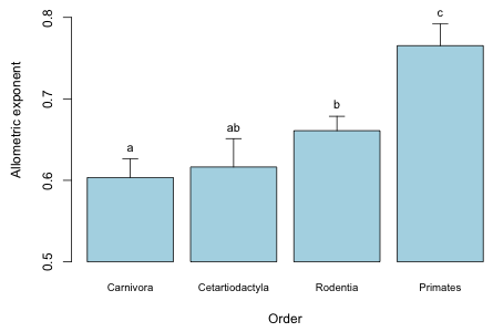
my.means
Carnivora Cetartiodactyla Rodentia Primates
0.6034166 0.6163946 0.6609356 0.7652427
# results of pairwise comparisons
diffs <- c('a','ab','b','c')
# rescale things for the plot
dat1 <- my.means-.5
# create bar plot and save coordinates of bars
bp <- barplot(dat1, axes=F, ylim=c(0,.35), names.arg=names(my.means), cex.names=0.8, ylab='Allometric exponent', xlab='Order',col='lightblue')
# add correct labels on y-axis (because of rescaling)
axis(2, at=seq(0,.3,.1), labels=seq(0,.3,.1)+.5)
# add handles to dynamite plot
arrows(x0=bp, y0=dat1, x1=bp, y1=dat1+se.mean.sort, angle=90, length=0.1)
# add labels to the handles
text(bp, dat1+se.mean.sort, diffs, pos=3, cex=.9)
|
| Fig. 1 Dynamite graph showing the pairwise comparisons of the allometric exponents by order. (No correction for multiple testing was made.) |
Graphical summary—confidence intervals
A more elegant way of summarizing things is is by plotting 95% confidence intervals for the allometric exponents by mammalian order along with suitable difference-adjusted confidence intervals. The easiest way to obtain the individual slopes is to fit a reparameterized version of the model in which the individual intercepts and slopes are returned for the four mammalian orders. The details of this were explained in lecture 8. The reparameterization needed for the current model is the following.
out2 <- lm(log(brain) ~ log(body):sp.order + sp.order-1, data=brainbody)
round(summary(out2)$coefficients,3)
Estimate Std. Error t value Pr(>|t|)
sp.orderCarnivora -1.348 0.232 -5.803 0.000
sp.orderCetartiodactyla -1.176 0.397 -2.966 0.003
sp.orderPrimates -2.000 0.207 -9.668 0.000
sp.orderRodentia -2.546 0.089 -28.586 0.000
log(body):sp.orderCarnivora 0.603 0.023 26.315 0.000
log(body):sp.orderCetartiodactyla 0.616 0.035 17.784 0.000
log(body):sp.orderPrimates 0.765 0.027 28.603 0.000
log(body):sp.orderRodentia 0.661 0.018 37.561 0.000
The slopes appear in rows 5 through 8 of the output. To obtain the 95% confidence intervals we can use the confint function on the model.
confint(out2)
2.5 % 97.5 %
sp.orderCarnivora -1.8041545 -0.8919669
sp.orderCetartiodactyla -1.9551127 -0.3974975
sp.orderPrimates -2.4066510 -1.5941133
sp.orderRodentia -2.7206716 -2.3709385
log(body):sp.orderCarnivora 0.5583916 0.6484416
log(body):sp.orderCetartiodactyla 0.5483393 0.6844499
log(body):sp.orderPrimates 0.7127109 0.8177745
0.6263849 0.6954863
To obtain the difference-adjusted confidence levels we need the ci.func function from lecture 5.
# function to calculate difference-adjusted confidence intervals
ci.func <- function(rowvals, lm.model, glm.vmat) {
nor.func1a <- function(alpha, model, sig) 1-pt(-qt(1-alpha/2, model$df.residual) * sum(sqrt(diag(sig))) / sqrt(c(1,-1) %*% sig %*%c (1,-1)), model$df.residual) - pt(qt(1-alpha/2, model$df.residual) * sum(sqrt(diag(sig))) / sqrt(c(1,-1) %*% sig %*% c(1,-1)), model$df.residual, lower.tail=F)
nor.func2 <- function(a,model,sigma) nor.func1a(a,model,sigma)-.95
n <- length(rowvals)
xvec1b <- numeric(n*(n-1)/2)
vmat <- glm.vmat[rowvals,rowvals]
ind <- 1
for(i in 1:(n-1)) {
for(j in (i+1):n){
sig <- vmat[c(i,j), c(i,j)]
#solve for alpha
xvec1b[ind] <- uniroot(function(x) nor.func2(x, lm.model, sig), c(.001,.999))$root
ind <- ind+1
}}
1-xvec1b
}
The variances and covariances of the slopes occupy rows 5 through 8 and columns 5 through 8 of the variance-covariance matrix of the model.
vals1 <- ci.func(1:4, out2, vcov(out2)[5:8,5:8])
vals1
[1] 0.8429977 0.8357554 0.8381188 0.8379638 0.8554106 0.8432272
Although the confidence levels don't vary much the little bit of variability that is shown does make a difference because the p-value for testing that the slopes of carnivores and rodents are equal is very close to 0.05. The confidence level for this comparison is the third element of vals1. I begin with the highest reported confidence level and obtain the corresponding confidence intervals using the confint function.
confint(out2, level=vals1[5])[5:8,]
7.23 % 92.77 %
log(body):sp.orderCarnivora 0.5699234 0.6369098
log(body):sp.orderCetartiodactyla 0.5657697 0.6670196
log(body):sp.orderPrimates 0.7261653 0.8043201
log(body):sp.orderRodentia 0.6352340 0.6866371
With this choice the interval for Primates doesn't overlap any of the others. But notice that the intervals for carnivores and rodents overlap. We know from the summary table of the original model that these two orders are just barely significantly different. Of course we're using the wrong difference-adjusted level for this comparison. I redo the calculations using the correct confidence level for this comparison.
confint(out2, level=vals1[3])[5:8,]
8.09 % 91.91 %
log(body):sp.orderCarnivora 0.5713061 0.6355271
log(body):sp.orderCetartiodactyla 0.5678596 0.6649296
log(body):sp.orderPrimates 0.7277786 0.8027068
log(body):sp.orderRodentia 0.6362950 0.6855761
Now the two intervals don't overlap. Because the conclusions for the rest of the comparisons remain the same, I use this level to calculate the difference-adjusted confidence intervals. I assemble everything in a data frame.
out838 <- confint(out2,level=vals1[3])[5:8,]
out95 <- confint(out2,level=.95)[5:8,]
newdata <- data.frame(var.labels=levels(brainbody$sp.order), ests=coef(out2)[5:8], out95, out838)
names(newdata)[3:6] <- c('low95', 'up95', 'low83', 'up83')
rownames(newdata)<-NULL
newdata
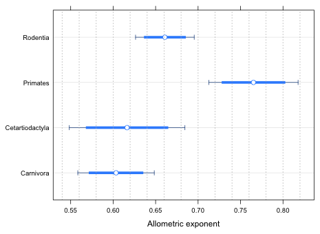
var.labels ests low95 up95 low83 up83
1 Carnivora 0.6034166 0.5583916 0.6484416 0.5713061 0.6355271
2 Cetartiodactyla 0.6163946 0.5483393 0.6844499 0.5678596 0.6649296
3 Primates 0.7652427 0.7127109 0.8177745 0.7277786 0.8027068
4 Rodentia 0.6609356 0.6263849 0.6954863 0.6362950 0.6855761
I modify the code from lecture 4 (for plotting effect estimates from regression models) for use here.
prepanel.ci <- function(x, y, lx, ux, subscripts, ...){
list(xlim=range(x, ux[subscripts], lx[subscripts], finite=T))}
dotplot(var.labels~ests, data=newdata, lx=newdata$low95, ux=newdata$up95, xlab='Allometric exponent', prepanel=prepanel.ci, panel=function(x,y){
panel.dotplot(x, y, col='white', cex=.01)
panel.arrows(newdata$low95, as.numeric(y), newdata$up95, as.numeric(y), col="dodgerblue4", angle=90,length=.05, code=3)
panel.segments(newdata$low83, as.numeric(y), newdata$up83, as.numeric(y), col="dodgerblue1", lwd=5, lineend=1)
panel.xyplot(x, y, pch=16, cex=1, col='white')
panel.xyplot(x, y, pch=1, cex=1.1, col='dodgerblue')
panel.abline(v=seq(0.54,0.84,.02), col='grey70', lty=3)
})
|
| Fig. 2 95% confidence intervals and difference-adjusted (83.8%) confidence intervals for the allometric exponents of four mammalian orders. The difference-adjusted intervals can be used to make pairwise comparisons among the orders. |
Question 6
I use tapply and the range function to obtain the ranges of the log body mass for each of the four mammalian orders.
out.r <- tapply(log(brainbody$body), brainbody$sp.order, range)
out.r
$Carnivora
[1] 4.838924 14.511902
$Cetartiodactyla
[1] 7.599401 17.876970
$Primates
[1] 3.988984 11.656124
$Rodentia
[1] 1.856298 9.806426
The output is a list. To extract the minimum value for Primates, e.g., I can write: out.r[[3]][1] because Primates are the third element in the list and the minimum is the first element of the Primate vector. To generate the plot of the regression lines restricting the ranges to the data for the separate orders I use the curve function. The coefficient vector of the model is the following.
coef(out1)
(Intercept) log(body)
-1.34806072 0.60341658
sp.orderCetartiodactyla sp.orderPrimates
0.17175561 -0.65232139
sp.orderRodentia log(body):sp.orderCetartiodactyla
-1.19774436 0.01297802
log(body):sp.orderPrimates log(body):sp.orderRodentia
0.16182611 0.05751898
The equation of the regression line for carnivores is
coef(out1)[1] + coef(out1)[2] * x.
For the three remaining orders the equation of the regression line takes the following form.
coef(out1)[1]+coef(out1)[y]+(coef(out1)[2]+coef(out1)[y+3])*x
where y is either 3, 4, or 5. Based on this I can write a function that draws the curve for Cetartiodactyla, Primates, and Rodentia.
mycurve <- function(y) curve(coef(out1)[1] + coef(out1)[y] + (coef(out1)[2] + coef(out1)[y+3])*x, from=out.r[[y-1]][1], to=out.r[[y-1]][2], col=mycol[y-1], lty=2, add=T)
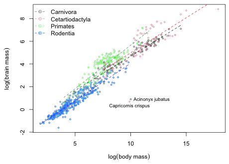
plot(log(brain)~log(body), data=brainbody, xlab=expression(log('body mass')), ylab=expression(log('brain mass')), col=c('grey50', 'pink2', 'lightgreen', 'dodgerblue1')[as.numeric(sp.order)], cex=.5)
# colors for lines
mycol <- c(1,2,'seagreen',4)
# draw Carnivora line
curve(coef(out1)[1] + coef(out1)[2]*x, from=out.r[[1]][1], to=out.r[[1]][2], col=mycol[1], lty=2, add=T)
# draw remaining lines: assign output of sapply to an object to suppress printing
junk <- sapply(3:5, mycurve)
legend('topleft', levels(brainbody$order), pch=1, col=c('grey50', 'pink2', 'lightgreen', 'dodgerblue1'), lty=2, bty='n')
identify(log(brainbody$body), log(brainbody$brain), brainbody$species, cex=.8)
|
| Fig. 3 Plot of the allometric relationship between brain mass and body mass on a log-log scale. |
Question 7
I used the identify function to add the names of the outlier species to the graph of Question 6. They are Acinonyx jubatus and Capricornis crispus.
Course Home Page