The data are drawn from an experiment in which a continuous response was measured for twelve treatment groups that were constructed by combining the levels of three categorical factors. Typically such an experiment is analyzed as a three-factor analysis of variance (ANOVA). Here's a description of the variables as supplied to me by the researcher.
Response: The response variable is mitotic activity in the intestine of my tadpoles after I fed them certain diets. I measured it using an antibody against phosphorylated histone (DNA histones are phosphorylated during mitosis), and basically it gives me a measure of how well the tadpoles are assimilating the diet that I feed them.
Factor 1 (Co, No and Ru) is a hormonal manipulation. In a previous experiment I found that these tadpoles exhibited more mitotic activity when fed shrimp (their native diet) and less when fed detritus. I was trying to figure out whether the reduction in mitotic activity on detritus was related to stress hormones. Co = CORT, or corticosterone, No = None, or control and Ru = Ru486, which is a CORT antagonist. So the thought was that if the depression of mitotic activity in detritus-fed tadpoles was alleviated by Ru486, or the elevated mitotic activity in shrimp-fed tadpoles was depressed by CORT, then stress hormones may be the proximate cause of diet-induced differences in these tadpoles.
Factor 2 is the diet. D = Detritus and S = Shrimp. Most tadpoles eat detritus, this species has evolved a novel diet of shrimp and other tadpoles.
Factor 3 is family. I used two sibships for this experiment, and, as I unfortunately found out, one of the families performed about as well on detritus as it did on shrimp (contrary to all other experiments I've done). So, there appears to be family variation for shrimp assimilation.
When R is launched the R Console window appears in which R commands can be entered. In the Windows operating system to move around within a command line to correct mistakes you need to use the left and right arrow keys on the keyboard rather than the mouse. The home and end keys can be used to move to the beginning and end of the current line. Previously issued commands can be recalled with the up arrow key. Choose Help > Console from the menu (Windows OS) for additional details. These same keyboard manipulations work with R for Mac OS X but in addition the mouse can be used to move around within the same command line.
Today's data set is tadpoles.csv. It is a comma-delimited text file. For purposes of this exercise you can download the file to your own computer and then read it into R or read it into R directly from the web site. I illustrate both methods.
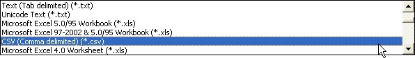
To read your own data into R from Excel, say, you would first need to create an appropriate text file. While there exist R packages for reading Excel files directly (on Windows machines), for most purposes it is preferable to use Excel to create a text file of your data and read in the text file instead. To create a text file from an Excel worksheet you would first choose File > Save As... from the file menu. In the Save As window that appears change the Save as type option at the bottom of the window to Text (tab delimited) (*txt) or CSV (Comma delimited) (*.csv). Fig. 1 shows both of these options with the comma-delimited option highlighted.
Fig. 1 Choosing the file format when saving files in Excel
The data set tadpoles.csv was created in this fashion. Here's a portion of what that file looks like when opened with a text editor.
response,treatment,fac1,fac2,fac3
,RuS1,Ru,S,1
,RuS1,Ru,S,1
,RuS1,Ru,S,1
,RuS1,Ru,S,1
The first row of the file contains the variable names separated by commas. The data values begin in row 2. The values of the variable "response" are missing for the first few observations so the first entry in these lines is a comma. One of the reasons for saving Excel files in a delimited format is so that missing observations are accounted for properly.
Save the tadpoles.csv file to a folder on your computer. This could be a specified folder that you've designated for work related to this class. Keep track of the full path name to the location of this file on your computer so that you can locate it again. The basic way to read data into R from a text file is to use the read.table function. R uses standard mathematical notation f(x,y,z) to specify functions and their arguments, so parentheses are always required with functions but for some functions it is not always necessary to specify arguments.
The structure of the current data file is such that we only need to specify three arguments.
The read.table function processes the external data file and creates an R object called a data frame which by default is then printed to the screen. To be able to retain function output we need to explicitly assign the output to a named R object using the assignment operator (also called the assignment arrow). The assignment arrow is constructed from two keyboard characters and is either a left-pointing arrow, <- , or a right-pointing arrow, ->. The arrow points in the direction of the assignment.
Note: The <- can be replaced with an = sign. The equal sign always assigns the result of the calculation on the right to the variable on the left of the equal sign. Thus it cannot be used to replace ->.
The following line reads in the data file from the specified location on my computer and stores the result in an object called tadpoles.
Windows uses a single back slash, \, to separate the folders in the path name of a file. This representation is not allowed in R. You should replace each back slash with a forward slash, as in the URLs of web sites, or with double back slashes. For example, if the file tadpoles.txt is located on the C: drive in the folder ecol 563 of the Documents folder on my hard drive, I would specify the path name to this file using forward slashes as follows.
'C:/Users/jmweiss/Documents/ecol 563/tadpoles.csv'
Using double back slashes it would be the following.
'C:\\Users\\jmweiss\\Documents\\ecol 563\\tadpoles.csv',
You must not use the single backslashes that Windows conventionally uses as in 'C:\Users\jmweiss\Documents\ecol 563\tadpoles.csv'. The single backslash is used within character strings to denote special characters in R and modifies how text enclosed in quotes will print to the screen.
In Mac OS X the file name syntax is a little different. Suppose I have the file in a folder I call ecol563 in the Documents folder on my hard disk. The correct file designation for me would be:
'/Users/jackweiss/Documents/ecol563/tadpoles.csv'.
You can see the path name for a file by clicking on the folder name at the top of its window while holding down the command (apple) key. In specifying the path in R it is not necessary to include any details about the path for any folder in the hierarchy that is above the Users folder.
Mac OS X also supports file drag and drop. For instance, you can type read.table("", header=T, sep=',') leaving out the file name, drag the icon of the data file from its source folder to the R console window, and release it when the cursor lies between the quotation marks. The file name with the complete correct path designation will appear between the quotation marks. Make sure there are no extra spaces inside the quotes before you press the return key.
Remember that the files created by programs such as Excel, Notepad, Textedit, etc. have extensions associated with them by default. You will not see those extensions if your operating system is configured so that file extensions are made invisible, but they are still there. Typically they will be .txt (for space-delimited or tab-delimited files), .dat (sometimes for tab-delimited files), and .csv (for comma-delimited files). If you get an error message such as 'No such file or directory' with the read.table function it may be because you did not include the extension in the file name.
Anytime you get an error message resembling the one shown above, it means you've made an error in specifying the name or location of the file. R treats any line that begins with a # symbol as a comment and ignores it. I will occasionally mix comments in with the code to annotate what's being done. They will be colored green with a shaded background.
A problem with some operating systems is that the details of the file hierarchy are concealed from the user so that a file's exact address may be unclear. Here are a couple of work-arounds if that is the case.
You don't have to know the location of the file to read it into R. You can use the file.choose function for the file location in read.table. This will bring up a "File Choose" window within which you can then navigate to the file.
I don't recommend this as a regular option. Ideally you want to save all of the R commands used for an analysis in a text file so that you can easily repeat the analysis when needed. Having to negotiate through a file selection window each time is silly, particularly when at a future date you may not even remember the name of the data file you used in the analysis. I recommend hard-wiring the file location in.
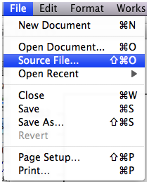
Fig. 2 Source file… in File menu
Depending on the operating system you're using the full path to files in special folders may not be explicitly shown (e.g., in older versions of Windows). In this case you can use R to show you the path name of your file. Use Notepad to create a text file with a single calculation line in it, say the mathematical expression 2+2. Save this file in the same folder containing your data. For instance, I save it as the file arithmetic.txt.
Next within R choose File > Source File … (Fig. 2) from the menu, navigate to the folder that contains the file you just created, change the file type in the drop-down menu to All files (*.*), and select it. R will display the entire path name of the file it is sourcing in the console window.
source("C:\\Users\\jmweiss\\Documents\\ecol 563\\arithmetic.txt")Now all that's left to do is to copy this line (or use the up arrow on the keyboard to navigate to it), change the function name from source to read.table, change arithmetic.txt to the file name of the data set, and add the additional arguments header = T and sep=','.
Another thing that may help is to determine the folder that R is using as the current working directory. The working directory is the folder that R uses by default for reading and writing files. The getwd function of R returns the location of the working directory.
getwd()If the data file of interest happens to lie inside the Documents folder then just complete the rest of the path name. In fact because the Documents folder is the default working directory, you don't really need to give the full path to the file. You can start instead with the first folder inside the Documents folder that contains the file.
The read.table function is a general function that can be used to read in text files with various delimiters depending on the value that you specify in the sep argument. As we've seen sep=',' is used for comma-delimited files. To read in a tab-delimited file we would need to enter sep='\t'. If you leave off the sep argument entirely R assumes the values in the file are separated by spaces.
R also provides functions specific for comma-delimited and tab-delimited files: read.csv for comma-delimited files and read.delim for tab-delimited files. Both of these functions expect that the variable names appear in row 1 of the file so the header=T argument can be left off also. To read in the tadpoles file using read.csv we can do the following.
The read.table function can also be used to read in files from the web. For this the first argument of read.table is the URL of the file, where the entire URL is enclosed in quotes. This will work for files located on web sites whose URL begins with 'http://'. Unfortunately the Sakai site where the class files are stored is a secure site whose URL begins with "https://". Reading in public files from such sites is a two-step process in R that requires the use of the getURL function that is contained in the RCurl package. The RCurl package is not part of the standard installation of R so we'll first need to download it from the CRAN site and install it into our copy of R. This process needs to be done only once.
On Windows downloading and installing a new R package is a three-step process.
(a) 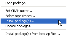 |
(b) 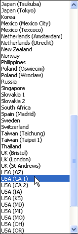 |
(c) 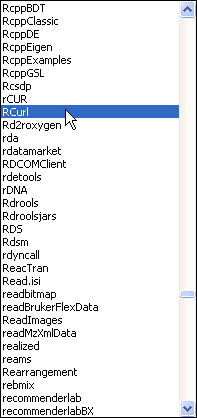 |
| Fig. 3 Windows OS: Installing an R package from the CRAN site on the web | ||
The desired package will be downloaded along with any additional packages it requires.
Choose Package Installer from the Packages & Data menu (Fig. 4a). In the window that appears (Fig. 4b) enter RCurl in the Package Search box and press the return key on the keyboard to search for the RCurl package. It should eventually appear in the Package column along with its version number. Click the Install Dependencies check box so that if the package depends on any other packages these will be downloaded also. Finally, highlight the desired package in the list (sometimes multiple packages appear) and click Install Selected to download the package to the R libraries folder.
(a) 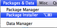 |
(b) 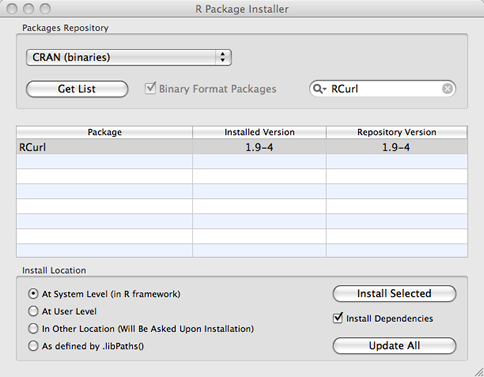 |
|
| Fig. 4 Mac OS X: Installing an R package from the CRAN site. | ||
If the package fails to turn up when searching for it, the CRAN mirror you're using doesn't have the appropriate version of the package for your installed version of R. In that case you can try changing the mirror by entering chooseCRANmirror() at the R command prompt in the console, choosing a different mirror site in the pop-up menu that appears, and repeating the above protocol to try to install the package again from the new site.
The package is now installed into your version of R but it hasn't been loaded into memory yet. That can be done with the library function.
The next step is to bring the text file into R from the web site with the getURL function from the RCurl package. This brings the contents of the file into R as a single long character string. In the command shown below I enclose the URL of the tadpoles.csv data set from the Sakai web site in quotes and make it the first argument of getURL. (I obtained the URL by right-clicking on the file and choosing "copy link location" from the context menu that appears.)
The above function call works on my Mac, but on Windows I get the following error message.
Error in function (type, msg, asError = TRUE) :I was able to fix this by adding two additional arguments to getURL, ssl.verifyhost=F and ssl.verifypeer=F.
Finally we need to convert the output from getURL into a usable format. The function textConnection will do this and the output from it can then be used as the first argument of read.table.
If you accidentally hit the return key before you finished typing a line, R will present you with a + prompt indicating that it is waiting for more information. At this point you can just finish the line and then hit return again. In line below I pressed the return key before closing the parenthesis on the read.table function.
> tadpoles <- read.table('ecol 563/tadpoles.csv', header=T, sep=','
+ )
Alternatively you can press the esc key to cancel the command altogether. Then you can then use the up arrow key, ↑, to move back to that line and finish it or fix any errors that you made.
Previously issued commands are stored in a history buffer. Accessing it is done differently in Windows and Mac OS X.
Old commands can be viewed by opening the history window. The command to do this is history(n) where n is the number of old command lines you wish to see. The following will retrieve the last 50 lines and display them in a separate window.
Eventually the history buffer gets filled and the old commands are lost, so you should issue this command frequently if you want to record your work. I usually paste the commands from the history window into a Notepad or Word document where I remove the mistakes and add comments. The contents of the history window can also be saved to a file by choosing File > Save to File ... from the menu when the R History window is the active window.
In Mac OS X the command history is displayed by clicking the history icon ![]() that appears in the tool bar at the top of the console window. This causes the list of old commands to appear on the right side of the console. A button at the bottom of this window can be used to save the entire history to a file.
that appears in the tool bar at the top of the console window. This causes the list of old commands to appear on the right side of the console. A button at the bottom of this window can be used to save the entire history to a file.
The object tadpoles created above with the read.table function is called a data frame. Data frames look like matrices but the elements of data frames can be mixtures of character and numeric data. More formally data frames are tightly coupled collections of variables that share many of the properties of matrices and of lists (another R data structure). Data frames are the fundamental data structures for most of R's modeling functions.
The dim function is used to determine the dimensions of a data frame.
The displayed output from dim is a vector with two components (the number of rows followed by the number of columns). From the output we see that there are 270 rows and 5 columns. We can view the beginning and the end of data frames with the head and tail functions of R.
Notice that the missing values in the original file have been replaced by the entry NA which stands for "not available". More generally we can access specific rows and columns of a data frame using bracket notation. To view the first six rows, denoted 1:6, and all columns I enter
To see only specific columns we need to enter those column numbers after the comma inside the brackets. To see only columns 1:2 of the first six rows the following will work.
To see all the values of the variable "response" we can access it by specifying column 1 of the data frame or by specifying the name of the column. To see all the observations I don't enter anything in the row position in front of the comma.
Variables can also be accessed from a data frame by using what's called list notation. For this we specify the name of the data frame, tadpoles, followed by a dollar sign, $, followed by the variable name.
The names function displays the names of the variables contained in a data frame.
Objects in R have a class attribute that can be extracted with the class function.
The variable "response" is identified as numeric variable while "treatment" is a factor. In the raw data file the "treatment" field consisted of character data. When R reads in a character variable it assumes that you plan to use the variable in regression models and so has converted it to a factor. It still has its original values but R has also created a set of dummy variables corresponding to the distinct values of the character variable. You can view the default coding system R has used with the contrasts function.
Because there are 12 different treatments R has created 11 dummy variables. It ordered the values of the character variable alphabetically and made the alphabetically first character value the reference level, in this case CoD1. The dummy variables are the columns shown in the output. Each indicates one of the remaining 11 levels. Similarly the variables fac1 and fac2 were converted to factors with associated dummy coding schemes.
Here we see that the columns labeled No and Ru are the dummy variables that indicate the No and Ru categories respectively. Recall from the researcher's description of the experiment that "No" is the control level of factor 1. Given this we might prefer to have "No" as the reference level. To accomplish this we would need to use the factor function with the levels argument in which we list the levels in the order we want specifying the reference level first.
If we examine the variable fac3, R tells us it's an integer variable. R has not converted it into a factor because the categories of this variable are numbers.
To convert this variable into a factor explicitly we can use the factor function. In the line below I create a new variable in the tadpoles data frame called fac.f that is the factor version of fac3.
Alternatively, we could just overwrite the old variable and replace it with its factor version.
One way to analyze these data is with a one-way analysis variance in which we parameterize the 12-category treatment variable with 11 dummy regressors. This is called the cell means model. Because analysis of variance is simply regression with dummy variables we can fit this model with lm, the ordinary linear regression function of R. lm stands for "linear model". The model can be fit as follows.
All regression models in R are fit using formula notation. To the left of the ~ is the response variable. To the right of the ~ is the linear model containing the predictors. The required notation is the response variable, followed the formula symbol ~, followed by the predictors separated by + signs if there is more than one. Because the variable treatment is of class factor, R will supply the eleven dummy variables required to fit the regression model for us.
A second way to analyze the data is to make use of the fact that the 12 treatments really are made up of three factors combined in all possible ways and carry out what's called a three-factor analysis of variance. With three factors the full three-factor analysis of variance includes the three main effects, the three two-factor interactions, and the single three-factor interaction.
The terms separated by colons are interactions. Thus, e.g., fac1:fac2 is the two-factor interaction between fac1 and fac2, and fac1:fac2:fac3 is the three-factor interaction. Different predictors are separated by + symbols.
R supports simpler notation for fitting this model. The notation fac1*fac2*fac3 is shortcut notation for a three-factor interaction plus all the terms to which it is marginal.
A second shortcut notation for fitting all combinations of fac1, fac2, and fac3 up to a three-factor interaction is the following.
The cell means (one-way ANOVA) model and the full factorial (three-way ANOVA) model are identical except for their parameterizations. This is apparent when we look at the summary output from these two models.
Residuals:
Min 1Q Median 3Q Max
-0.6594 -0.1382 -0.0095 0.1240 1.0555
Coefficients:
Estimate Std. Error t value Pr(>|t|)
(Intercept) 3.39846 0.06834 49.726 < 2e-16 ***
factor(treatment)CoD2 0.08071 0.09079 0.889 0.374927
factor(treatment)CoS1 -0.03242 0.08486 -0.382 0.702785
factor(treatment)CoS2 0.30708 0.08486 3.619 0.000365 ***
factor(treatment)NoD1 0.51180 0.08869 5.770 2.58e-08 ***
factor(treatment)NoD2 0.65571 0.08486 7.727 3.52e-13 ***
factor(treatment)NoS1 0.57522 0.08620 6.673 1.90e-10 ***
factor(treatment)NoS2 0.82191 0.08486 9.686 < 2e-16 ***
factor(treatment)RuD1 0.53737 0.09865 5.447 1.33e-07 ***
factor(treatment)RuD2 0.62154 0.08486 7.324 4.15e-12 ***
factor(treatment)RuS1 0.74804 0.09865 7.583 8.58e-13 ***
factor(treatment)RuS2 0.95041 0.08486 11.200 < 2e-16 ***
---
Signif. codes: 0 ‘***’ 0.001 ‘**’ 0.01 ‘*’ 0.05 ‘.’ 0.1 ‘ ’ 1
Residual standard error: 0.2464 on 227 degrees of freedom
(31 observations deleted due to missingness)
Multiple R-squared: 0.6264, Adjusted R-squared: 0.6083
F-statistic: 34.6 on 11 and 227 DF, p-value: < 2.2e-16
Residuals:
Min 1Q Median 3Q Max
-0.6594 -0.1382 -0.0095 0.1240 1.0555
Coefficients:
Estimate Std. Error t value Pr(>|t|)
(Intercept) 3.398462 0.068344 49.726 < 2e-16 ***
fac1No 0.511802 0.088695 5.770 2.58e-08 ***
fac1Ru 0.537372 0.098646 5.447 1.33e-07 ***
fac2S -0.032420 0.084859 -0.382 0.7028
fac32 0.080715 0.090790 0.889 0.3749
fac1No:fac2S 0.095839 0.114704 0.836 0.4043
fac1Ru:fac2S 0.243087 0.131610 1.847 0.0660 .
fac1No:fac32 0.063189 0.118189 0.535 0.5934
fac1Ru:fac32 0.003452 0.125829 0.027 0.9781
fac2S:fac32 0.258785 0.115338 2.244 0.0258 *
fac1No:fac2S:fac32 -0.155995 0.155945 -1.000 0.3182
fac1Ru:fac2S:fac32 -0.140577 0.168770 -0.833 0.4057
---
Signif. codes: 0 ‘***’ 0.001 ‘**’ 0.01 ‘*’ 0.05 ‘.’ 0.1 ‘ ’ 1
Residual standard error: 0.2464 on 227 degrees of freedom
(31 observations deleted due to missingness)
Multiple R-squared: 0.6264, Adjusted R-squared: 0.6083
F-statistic: 34.6 on 11 and 227 DF, p-value: < 2.2e-16
Observe that all of the summary statistics reported at the bottom of the output are the same for the two models. Although each model uses 12 parameters to describe the outcome, the parameter estimates are different. The problem with the cell means model is that it is overly complicated. The summary output of the cell means model allows one to test whether individual treatment means are different from the reference group treatment mean (CoD1). Of the 11 tests reported, nine of them are statistically significant. Now, if these were the only tests we were interested in then the one-way model has been a success. But with 12 treatments there are 66 (= 12 × 11 ÷ 2) possible pairwise comparisons we can make. The task of summarizing all these tests is an organizational mess. Furthermore by carrying out so many tests each at significance level α = .05, we are guaranteed that some of these tests (on average 66 × .05 = 3.3) will yield significant results just by chance, i.e., we'll reject the null hypothesis when in fact the null hypothesis is true.
It's almost never a good strategy to fit the cell means model first. If the treatments possess a structure then it makes sense to take advantage of it. When treatments are constructed by combining factors in all possible ways, analyzing it as a factorial design instead allows us to tease apart the independent effects of the individual factors (main effects) as well as the synergistic effects (interactions) if present. The advantage of the factorial design is that it helps us understand the reasons why the means show the pattern they do. Furthermore if it turns out that the individual factors affect the response in a simple fashion, we will be able to parsimoniously describe the response with fewer than twelve parameters. In the end it will still be possible to obtain the individual treatment means if they are desired. On the other hand, if it turns out that the three-factor interaction is statistically significant, then nothing will have been gained (or lost) by analyzing the data with a three-way ANOVA model. In that case the treatment differences fail to exhibit a pattern in terms of their component factors.
When analyzing categorical regression models it is necessary to distinguish the categorical variables themselves (the predictors) from the dummy variables (regressors) that we use to represent them in the regression model. The regressors that correspond to a single categorical variable or effect are a unit that is sometimes referred to as a construct (Polissar and Diehr 1982). To simplify the regression model, we try to drop constructs, not individual dummy regressors. R's anova function allows us to examine the statistical significance of the individual model constructs. When dealing with an experiment in which the experimental units have been randomly assigned to treatments the full interaction model is the right place to begin the analysis.
Response: response
Df Sum Sq Mean Sq F value Pr(>F)
fac1 2 18.4339 9.2169 151.7899 < 2.2e-16 ***
fac2 1 1.5013 1.5013 24.7238 1.304e-06 ***
fac3 1 2.2771 2.2771 37.5007 3.984e-09 ***
fac1:fac2 2 0.3926 0.1963 3.2328 0.04127 *
fac1:fac3 2 0.0838 0.0419 0.6900 0.50263
fac2:fac3 1 0.3503 0.3503 5.7693 0.01711 *
fac1:fac2:fac3 2 0.0695 0.0347 0.5723 0.56505
Residuals 227 13.7838 0.0607
---
Signif. codes: 0 ‘***’ 0.001 ‘**’ 0.01 ‘*’ 0.05 ‘.’ 0.1 ‘ ’ 1
The last column reports p-values for the F-statistics (labeled F value in the output). Each test is a sequential test. It tests whether the effect in a given row is statistically significant when added to a model that already contains all the terms listed above it in the table. For the test to make sense it must adhere to the principle of marginality, something that the anova function does. (According to the principle of marginality models with two-factor interactions must include all the component main effect terms that make up the interactions. Furthermore if a three-factor interaction is in the model then the three two-factor interactions and three main effects to which the three-factor interaction is marginal must also be in the model.)
The important conclusion that we can draw from the anova output above is that the three-factor interaction is not statistically significant (as seen from the p-value p = 0.565 in the row labeled fac1:fac2:fac3). Because the tests are carried out sequentially and knowing that the three-factor interaction is not significant, it is legitimate to examine the tests of two-factor interactions that appear in the table. From the output it appears that the fac1:fac3 interaction is not significant, but the the remaining two are. We need to be careful though. In unbalanced designs (unequal numbers of observations per treatment) such as this one, context matters. In a sequential ANOVA table changing the order in which the terms are listed will lead to different results when the design is unbalanced.
Sequential tests such as those produced by the anova function are called Type I tests. Type II tests (carried out by the Anova function of the car package) are generally considered preferable with unbalanced data. The car package is not part of the standard R installation so it must first be downloaded from the CRAN site, a process that was described for the RCurl package above.
Response: response
Sum Sq Df F value Pr(>F)
fac1 18.0783 2 148.8618 < 2.2e-16 ***
fac2 1.6498 1 27.1702 4.184e-07 ***
fac3 2.2300 1 36.7243 5.609e-09 ***
fac1:fac2 0.2997 2 2.4681 0.08702 .
fac1:fac3 0.0550 2 0.4525 0.63659
fac2:fac3 0.3503 1 5.7693 0.01711 *
fac1:fac2:fac3 0.0695 2 0.5723 0.56505
Residuals 13.7838 227
---
Signif. codes: 0 ‘***’ 0.001 ‘**’ 0.01 ‘*’ 0.05 ‘.’ 0.1 ‘ ’ 1
The last two tests reported by anova and Anova are the same, but the remaining tests are different. Anova tests a term in a model after first removing any terms that the term of interest is marginal to. A marginal term is one that is properly contain in another. For instance, the main effect fac2 is contained in the terms fac1:fac2, fac2:fac3, and fac1:fac2:fac3. In the Anova function the Type II test of fac2 involves a model in which these three terms have been removed. As a result we compare the following two models.
tadpoles ~ fac1 + fac3 + fac1:fac3 + fac2
tadpoles ~ fac1 + fac3 + fac1:fac3
except that we use as our measure of the background variation the residual sum of squares of the three-factor interaction model out1. On the other hand the Type I test of fac2 from the anova function would compare the following two models.
tadpoles ~ fac1 + fac2
tadpoles ~ fac1
once again using the residual error of the three-factor interaction model as a measure of background variation.
The Type I and Type II tests of the term fac1:fac3 differ in that the Type II test only excludes the three-factor interaction from the models it compares (fac1:fac2:fac3 is marginal to fac1:fac3), while the Type I test, because of the way the terms were listed in the model formula, excludes the three-factor interaction and the fac2:fac3 two-factor interaction. Because neither the Type I or Type II tests find fac1:fac3 to be statistically significant, we feel confident that we can drop it along with the three-factor interaction.
Based on our analysis above it appears we can drop the fac1:fac2:fac3 three-factor interaction and the the fac2:fac3 two-factor interaction. To do that we can use the long form of the model formula and omit those terms.
Alternatively, we can use the update function. With the update function we just subtract off the terms we want to remove from the full model.
The first argument is the model we want to update. The second argument begins with .~. which is a surrogate for the formula of model out1 from which we then subtract off the two terms shown.
Response: response
Df Sum Sq Mean Sq F value Pr(>F)
fac1 2 18.4339 9.2169 153.0824 < 2.2e-16 ***
fac2 1 1.5013 1.5013 24.9343 1.169e-06 ***
fac3 1 2.2771 2.2771 37.8201 3.382e-09 ***
fac1:fac2 2 0.3926 0.1963 3.2603 0.04015 *
fac2:fac3 1 0.3792 0.3792 6.2973 0.01278 *
Residuals 231 13.9083 0.0602
---
Signif. codes: 0 ‘***’ 0.001 ‘**’ 0.01 ‘*’ 0.05 ‘.’ 0.1 ‘ ’ 1
Response: response
Sum Sq Df F value Pr(>F)
fac1 18.0783 2 150.1294 < 2.2e-16 ***
fac2 1.6319 1 27.1043 4.258e-07 ***
fac3 2.2300 1 37.0370 4.777e-09 ***
fac1:fac2 0.3017 2 2.5057 0.08384 .
fac2:fac3 0.3792 1 6.2973 0.01278 *
Residuals 13.9083 231
---
Signif. codes: 0 ‘***’ 0.001 ‘**’ 0.01 ‘*’ 0.05 ‘.’ 0.1 ‘ ’ 1
The Type I and Type II tests disagree about the importance of the fac1:fac2 interaction. The sequential Type I test which tests fac1:fac2 in a model without the fac2:fac3 interaction finds it to be significant (p = 0.04) while the Type II tests which does include the fac2:fac3 in the reference model finds it to be not significant (p = 0.08). Of course the difference between these two p-values is rather small and the only reason we're having a discussion is because we've arbitrarily chosen α = .05 as the cut-off for statistical significance. Given that fac1 is the factor of primary interest to the researcher, we should probably examine the interaction fac1:fac2 further before deciding what to do about it.
Interactions can be examined graphically in a mean profile plot or what's sometimes called an interaction plot. These were discussed briefly in lecture 1. The effects package of R makes the generation of such a plot fairly easy. The effects package is not part of the standard R installation and it must first be downloaded from the CRAN site on the web. Before using the effects package the first time in a session it needs to be loaded into memory with the library function.
The function we need is called effect. It takes two required arguments:
We then plot the output from effect using the R plot function. I add the option multiline=T to get separate mean profiles displayed in the same panel.
Given the ambiguity of the results from the Type I and Type II tests it makes sense to examine the graphical evidence for a two-factor interaction between fac1 and fac2. There are two different ways that the two-factor interaction can be displayed and I present both. The plot method for an effect object allows the use of two additional keywords, x.var= and z.var=, that alter the factors displayed on the x-axis and the factor used to define the different profiles, respectively. Using these arguments I create an additional view of the two-factor interaction. Fig 5a displays fac1 on the x-axis and uses fac2 to distinguish the different profiles while Fig. 5b displays fac2 on the x-axis and uses fac3 to define the different profiles.
(a) 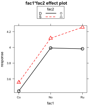 |
(b) 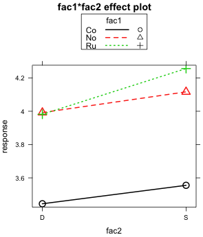 |
| Fig. 5 Two alternate graphical displays of the fac1 × fac2 two-factor interaction | |
What both graphs reveal is that if fac1 only consisted of the first two levels "Co" and "No", then there would clearly be no two-factor interaction to speak of. When restricted to just these two levels, the profiles are parallel. It's only when the third level "Ru" is included does the lack of parallelism become an issue.
The magnitudes of the effects shown in these plots are worth considering. Recall that "No" is the control group. So when the treatment "Co" is applied, the mean response decreases by 0.5 units regardless of the level of fac2 (Fig. 5b). On the other hand when "Ru" is applied , the response remains unchanged when fac2 is at level "D". But if fac2 is at level "S" the response increases by about 0.15 units. Observe that this "S" effect for "Ru" is about one third the magnitude of the "Co" effect. Given the large size difference in the effects, this raises the question of whether an effect so small is of much consequence.
We can get additional insight by looking at the summary table of a model containing the fac1:fac2 interaction.
summary(out2)
Call:
lm(formula = response ~ fac1 + fac2 + fac3 + fac1:fac2 + fac2:fac3)
Residuals:
Min 1Q Median 3Q Max
-0.67091 -0.13746 -0.01539 0.11680 1.07076
Coefficients:
Estimate Std. Error t value Pr(>|t|)
(Intercept) 3.38324 0.05245 64.499 < 2e-16 ***
fac1No 0.54730 0.05837 9.376 < 2e-16 ***
fac1Ru 0.53699 0.06085 8.825 2.76e-16 ***
fac2S 0.01715 0.06696 0.256 0.7981
fac32 0.10758 0.04815 2.234 0.0264 *
fac1No:fac2S 0.01341 0.07728 0.174 0.8623
fac1Ru:fac2S 0.16350 0.08175 2.000 0.0467 *
fac2S:fac32 0.16323 0.06505 2.509 0.0128 *
---
Signif. codes: 0 ‘***’ 0.001 ‘**’ 0.01 ‘*’ 0.05 ‘.’ 0.1 ‘ ’ 1
Residual standard error: 0.2454 on 231 degrees of freedom
Multiple R-Squared: 0.623, Adjusted R-squared: 0.6116
F-statistic: 54.53 on 7 and 231 DF, p-value: < 2.2e-16
The two lines I've colored in red contain estimates of the two dummy variables associated with the fac1:fac2 interaction. Both of these dummy variable estimates are interpretable in terms of what is shown in Fig. 5.
The output from model out2 tells us that we should not drop the fac2:fac3 interaction. (It was the last term added and it is significant at the α = .05 level, p = 0.013.) On the other hand what if we did choose to drop the fac1:fac2 interaction? This is model out3 below. The ANOVA table finds the fac1:fac2 interaction to be highly significant.
Response: response
Df Sum Sq Mean Sq F value Pr(>F)
fac1 2 18.4339 9.2169 151.1291 < 2.2e-16 ***
fac2 1 1.5013 1.5013 24.6162 1.350e-06 ***
fac3 1 2.2771 2.2771 37.3375 4.137e-09 ***
fac2:fac3 1 0.4700 0.4700 7.7069 0.005948 **
Residuals 233 14.2100 0.0610
---
Signif. codes: 0 ‘***’ 0.001 ‘**’ 0.01 ‘*’ 0.05 ‘.’ 0.1 ‘ ’ 1
So regardless of our decision about fac1:fac2, we should definitely retain the two-factor interaction fac2:fac3. I examine this interaction graphically using both possible ways of displaying it.
(a) 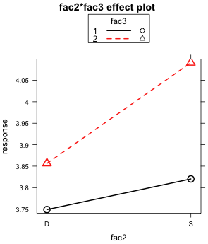 |
(b) 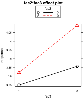 |
| Fig. 6 The two graphical displays of the fac2 × fac3 two-factor interaction | |
The lack of parallelism of the mean profiles is apparent in both plots.
The substantive meaning of a three-factor interaction can be assessed by examining plots of the two-factor interaction for two of the variables contained in the interaction at fixed values of the third variable. Because there are three factors involved, there are multiple ways to display the three-factor interaction plot.
For the first plot I let the effect function choose the default display.
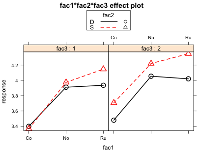
Fig. 7 Plot of the 3-factor interaction
Each panel is a plot of the same two-factor interaction plot, in this case the interaction between fac1 and fac2. The left panel shows this two-factor interaction when fac3 = 1 while the right panel shows the same two-factor interaction when fac3 = 2. If the nature of the two-factor interaction is different in these two panels then we have graphical evidence for the presence of a three-factor interaction. For example, if we saw evidence of a two-factor interaction in one panel but not in the other, then the nature of the two-factor interaction changes with the level of fac3 indicating that a three-factor interaction is probably present. Note that it's the pattern of the two-factor interaction that we're concerned with, not whether the two graphs are identical. If there are other two-factor interactions occurring between the variables, then it is unlikely that the two graphs will look the same.
So what do we learn from Fig. 7? I would argue that we get essentially the same pattern in both panels. If fac1 consisted only of levels Co and No we would fail to find evidence of a fac1 × fac2 interaction in either of the panels. In both panels the red and black profiles are roughly parallel. But when we add level Ru to the mix the profiles are no longer parallel. In both panels we see that the mean profiles diverge as we move from level No to level Ru. Both panels show roughly the same pattern so fac3 has failed to modify the nature of the two-factor interaction we're observing. Graphically then we do not find evidence of a three-factor interaction.
This is not the only three-factor interaction plot we could construct from these data. Currently fac1 is plotted on the x-axis, fac2 identifies the profiles, and fac3 defines the panels. These three assignments can be permuted in 2 × 2 × 2 = 6 different ways yielding six different ways of displaying the same three-factor interaction. Each version shows the same three-factor interaction but from a different perspective. All six plots should agree with each other but sometimes it is easier to draw conclusions from one plot than from another.
Using the arguments x.var and z.var I create two additional views of the three-factor interaction, one that uses the fac1:fac3 two-factor interaction (Fig. 8a) and the other the fac2:fac3 two-factor interaction (Fig. 8b). I start by creating the effect object and saving it as out2.eff, then I plot it using different settings for x.var and z.var.
(a) 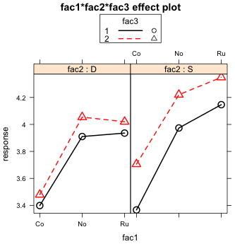 |
(b) 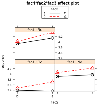 |
Fig. 8 Two additional graphical displays of the same three-factor interaction shown in Fig. 7 |
|
Fig 8a is more ambiguous than Fig. 7 was. If we look at the right panel of Fig. 8a when fac2 = 'S', we see that the two fac3 profiles are perfectly parallel. So there is clearly no evidence of a fac1 × fac3 interaction here. If we look at the left panel of Fig. 8a when fac2 = 'D', the fac3 profiles are not perfectly parallel (at least in the second half), but they're darn close. So this one is a tougher call but there is certainly no dramatic evidence of a fac1 × fac3 interaction. Because fac2 does not markedly affect the nature of the fac1 × fac3 interaction, we fail to find strong evidence of a three-factor interaction.
In Fig. 8b we see that the fac2 profiles are not perfectly parallel in any of the panels. While it is the case that the lack of parallelism is most pronounced when fac1 = Co, it never goes away. Thus there is evidence of the same fac2 × fac3 interaction in each panel. Because this interaction is not markedly affected by fac1, we fail to find evidence of a three-factor interaction using this plot either.
So we have two legitimate choices for the final model.
Choice 1 is a model that includes a two-factor interaction between factors 2 and 3 and only a main effect for factor 1.
Rationale: We tested for a three-factor interaction, fac1:fac2:fac3, and found it to be not statistically significant (p = 0.56). We then examined a model with all three two-factor interactions and sequentially dropped any two-factor interaction not significant at α = .05, starting with the least significant. Thus we dropped the fac1:fac2 interaction p = 0.635, followed by the fac1:fac3 interaction (p = 0.084). Examination of the fac1:fac3 interaction revealed that the effect was entirely due to level "Ru" of factor 1 having a larger effect than expected when factor 3 was at level "S". This effect was much smaller though than the main effect of level "No" and thus was not considered large enough to be of interest. The remaining two-factor interaction was highly significant (p = 0.006) as was the main effect of factor 1 (p < 0.001).
Choice 2 is a model that includes a two-factor interaction between factors 2 and 3 and a two-factor interaction between factors 1 and 3.
Rationale: We tested for a three-factor interaction, fac1:fac2:fac3, and found it to be not statistically significant (p = 0.56). We then switched to a main effects model and found that when we sequentially added two-factor interactions in the order fac1:fac3, fac2:fac3, and fac1:fac2 that fac1:fac3 was statistically significant (p = 0.040), fac2:fac3 was statistically significant (p = 0.013), but that fac1:fac2 was not (p = 0.635). I would argue that the rationale given here for this choice is pretty weak but the choice could be supported if the fac1:fac2 interaction had some special biological interest.
In the basic analysis of variance we assume that
![]()
where i denotes the treatment, j an experimental unit assigned to that treatment, and y is the response. So each observation has a normal distribution in which the mean, μi, varies by treatment i, but the variance, σ2, is the same for each observation. This is called the constant variance or homogeneity of variance assumption.
A convenient graphical way to compare the distributions of groups side by side is the box plot. We look first at the default display and then modify it incrementally to increase its information content. Here's the default box plot display we get of the distribution of the response variable for each treatment. The basic syntax for the boxplot function in R is to specify the response variable followed by a tilde, ~, which is the formula symbol in R, followed by the grouping variable.
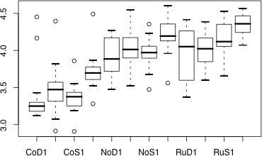
Fig. 9 Box plot of experiment results
The boxes themselves display the locations of the middle 50% of the data. The top and bottom edges are the first and third quartiles, Q1 and Q3, respectively. The horizontal line in each box is the location of the median. The whiskers on the boxes extend out to the smallest and largest values within the inner fences. The inner fences are given by Q1 – 1.5 × IQ, Q3 + 1.5 × IQ, where IQ is the interquartile width, Q3 – Q1. The small circles denote individual observations that lie beyond the inner fences.
One problem with this display is that there is not enough room to show all of the treatment labels on the x-axis. By default R suppresses the printing of some of the labels if they interfere with each other. One solution is to switch the x- and y-axes here so that the treatments appear on the y-axis, and then rotate the labels so that they are horizontal. Given that our final analysis will be a comparison of treatment means it would useful to add the mean of each group to the boxplot. With both the mean and median of each group visible we can also examine each distribution for skewness by seeing whether or not the median and mean occur at roughly the same place.
The boxplot function is an example of a higher level graphics function in R. By default, each call to boxplot opens up a new graphics window and erases the current display. R also provides lower level graphics functions that can be used to add information to plots that are currently being displayed. One of those lower level functions is points (to add additional plotted points to a display) which we can use to add the means to the display.
First we need to obtain the mean response of each treatment group. This can be obtained with the tapply function.
CoD1 CoD2 CoS1 CoS2 NoD1 NoD2 NoS1 NoS2
3.398462 3.479176 3.366042 3.705542 3.910263 4.054167 3.973682 4.220375
RuD1 RuD2 RuS1 RuS2
3.935833 4.020000 4.146500 4.348875
If we leave off the na.rm=T argument we get the missing code NA for some of the treatment groups.
Next I produce the boxplot, but I transpose the boxes with the horizontal=T option. The xlab= argument adds a label for the x-axis. The option las=1 makes the labels at the tick marks horizontal.
Next I use the points function to add the treatment means. Unlike boxplot, points does not support the tilde notation. Instead we have to enter the x-coordinates followed by the y-coordinates of the points separated by commas. The y-coordinates of the boxes (after rotation) are just the numeric values of the treatment factor, which are the numbers 1 through 12. I use an asterisk, pch=8, to denote the means and color them red, col=2.
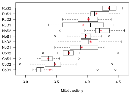
Fig. 10 Graphical summary of the results of the tadpole experiment
Fig. 10 highlights a potential problem with these data. Notice how the variability across the groups varies. In particular look at the RuD1 group. Its interquartile width is two to five times greater than that of any other group. This could mean that the treatment is affecting the variance in addition to the mean. It could also mean that a number of confounding factors have not been properly controlled for in this experiment thus introducing heterogeneity in the groups. In either case the observed heterogeneity of group variances calls into question the constant variance assumption.
Solutions to this problem are to use a distribution (other than the normal) in which the variance is allowed to vary. Another solution is to keep the normal distribution but to use generalized least squares (GLS) rather than ordinary least squares (OLS) to estimate the model. In GLS we can include an additional model for the variance. We'll revisit this issue later in the course.
Polissar, Lincoln and Paula Diehr. 1982. Regression analysis in health services research: the use of dummy variables. Medical Care 20(9): 959–966.
A compact collection of all the R code displayed in this document appears here.
| Jack Weiss Phone: (919) 962-5930 E-Mail: jack_weiss@unc.edu Address: Curriculum for the Environment and Ecology, Box 3275, University of North Carolina, Chapel Hill, 27599 Copyright © 2012 Last Revised--Aug 28, 2012 URL: https://sakai.unc.edu/access/content/group/3d1eb92e-7848-4f55-90c3-7c72a54e7e43/public/docs/lectures/lecture2.htm |