In simple linear regression we attempt to model the relationship between a single response variable y and a predictor x with an equation of the following form.
![]()
This is just the equation of a line with intercept β0 and slope β1 in which we account for the fact that the fit isn't perfect so that there is error represented by ε. Typically we assume that ![]() , i.e., that the errors are independent and are drawn from a common normal distribution. Equivalently we could also write
, i.e., that the errors are independent and are drawn from a common normal distribution. Equivalently we could also write
![]()
From this formulation we see that the regression line is the mean of the response variable y, i.e., ![]() , so that the mean changes depending on the value of x. The parameters of the regression model are typically estimated using least squares.
, so that the mean changes depending on the value of x. The parameters of the regression model are typically estimated using least squares.
To illustrate these ideas and to examine the typical linear regression output from statistical packages, I generate some random data, use it to construct a response variable, and finally estimate some simple linear regression models using R.
Individual regression lines of y versus x1 and y versus x3 are shown in Fig. 1. A horizontal line located at the mean of the response variable is included for reference. Without additional information or predictors, the sample mean of the response is the best predictor of a new value of y.
(a) 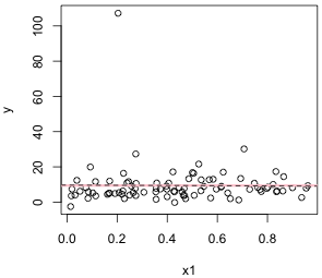 |
(b) 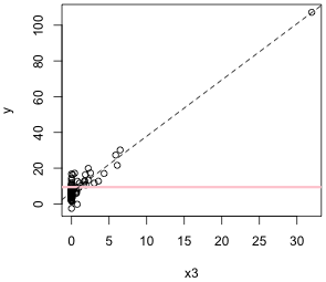 |
| Fig. 1 Individual regression lines for y versus (a) x1 and (b) y versus x2. The pink horizontal line denotes the response mean. The dashed line is the regression line. | |
From the graphs it would appear that y is linearly related to x3 but perhaps not to x1. (Observe also that it may be the case that a single point in Fig. 1b is having a profound effect on the location of the regression line.) To assess the fit of the lines we can examine the output from the regression.
Residuals:
Min 1Q Median 3Q Max
-12.178 -4.564 -1.986 1.389 97.676
Coefficients:
Estimate Std. Error t value Pr(>|t|)
(Intercept) 9.6623 2.4493 3.945 0.00016 ***
x1 -0.5975 4.8060 -0.124 0.90134
---
Signif. codes: 0 ‘***’ 0.001 ‘**’ 0.01 ‘*’ 0.05 ‘.’ 0.1 ‘ ’ 1
Residual standard error: 11.86 on 88 degrees of freedom
Multiple R-squared: 0.0001756, Adjusted R-squared: -0.01119
F-statistic: 0.01546 on 1 and 88 DF, p-value: 0.9013
The most useful features of the output are highlighted in yellow. We see that the estimated regression line is 9.66 – 0.60x1. The highlighted p-value in the column Pr(>|t|) is for a test of the null hypothesis that β1 = 0, i.e., that the slope of the regression line is zero. Because the reported p-value is large, p = 0.90, we fail to reject the null hypothesis. Hence we fail to find evidence that the response y is linearly related to the predictor x1. This is also confirmed by the statistic labeled "Multiple R-squared" a commonly-used goodness of fit statistic. For simple linear regression it is the square of the correlation coefficient between y and x1. It also measures the proportion of the original variability in the response that has been explained by the linear regression. In this case that proportion is almost zero telling us that the regression model is essentially worthless.
When we turn to the linear regression of y on x3, the results appear more promising.
Residuals:
Min 1Q Median 3Q Max
-9.0089 -2.4768 -0.3318 1.7561 10.3645
Coefficients:
Estimate Std. Error t value Pr(>|t|)
(Intercept) 6.3972 0.3965 16.13 <2e-16 ***
x3 3.1489 0.1080 29.16 <2e-16 ***
---
Signif. codes: 0 ‘***’ 0.001 ‘**’ 0.01 ‘*’ 0.05 ‘.’ 0.1 ‘ ’ 1
Residual standard error: 3.632 on 88 degrees of freedom
Multiple R-squared: 0.9062, Adjusted R-squared: 0.9051
F-statistic: 850.3 on 1 and 88 DF, p-value: < 2.2e-16
The reported regression line is 6.40 – 3.15x3. So, a one unit change in x3 yields a 3.15 unit change in the response. The reported p-value for the test of whether the slope is equal to zero is extremely small, reported as zero to 16 decimal places. So, we reject the null hypothesis and conclude that there is a significant linear relationship between y and x3. The reported R2 = 0.91 is also exceedingly high. It tells us that 91% of the original variability of the response is explained by its linear relationship with x3.
The reason that R2 is so high here is largely because of the outlier we observed in Fig. 1b. That point is a long way from the mean response and hence is a major contributor to the variability of the response. The fitted regression line passes almost exactly through this point so it contributes nothing to the variability about the regression line. Not surprisingly if we remove this point and refit the regression line to the remaining points, the reported R2 is much reduced.
Residuals:
Min 1Q Median 3Q Max
-9.0012 -2.4907 -0.3944 1.7376 10.3448
Coefficients:
Estimate Std. Error t value Pr(>|t|)
(Intercept) 6.4170 0.4250 15.10 <2e-16 ***
x3 3.1128 0.2894 10.76 <2e-16 ***
---
Signif. codes: 0 ‘***’ 0.001 ‘**’ 0.01 ‘*’ 0.05 ‘.’ 0.1 ‘ ’ 1
Residual standard error: 3.653 on 87 degrees of freedom
Multiple R-squared: 0.5708, Adjusted R-squared: 0.5658
F-statistic: 115.7 on 1 and 87 DF, p-value: < 2.2e-16
R2 is now reported to be 0.57. This tells us that R2 as a goodness of fit statistic is highly sensitive to outliers.
Of course just because a point is an outlier doesn't mean that it's also influential. If we compare the parameter estimates reported after removing the outlier to those that were obtained from fitting the model to the full data set, we see that they've barely changed.
When we include both lines in the same plot we see that they are nearly indistinguishable over the common range of the two data sets.
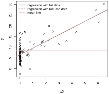 |
| Fig. 2 Comparison of the regression lines of y on x3 with and without an observation that is an outlier in x3-space. |
Multiple regression is really just a trivial extension of simple linear regression in which one predictor is replaced with multiple predictors. Excluding those situations where the additional predictor is just a function of the original predictor (such as in a quadratic model), a regression model with two predictors defines a plane in three-dimensional space. The geometric object defined by regression models with three or more predictors is called a hyperplane. Without a satisfactory way to visualize multiple regression models geometrically, we're forced to explore them analytically.
As an illustration I fit a linear regression model for y using the three predictors x1, x2, and x3. The regression model assumes the mean is given by
![]()
The output of special interest from this model is highlighted in yellow.
Residuals:
Min 1Q Median 3Q Max
-8.3681 -2.0349 -0.2121 1.6987 10.0899
Coefficients:
Estimate Std. Error t value Pr(>|t|)
(Intercept) 2.3468 1.5363 1.528 0.1303
x1 2.6665 1.4303 1.864 0.0657 .
x2 0.5756 0.2646 2.175 0.0324 *
x3 3.1128 0.1073 29.014 <2e-16 ***
---
Signif. codes: 0 ‘***’ 0.001 ‘**’ 0.01 ‘*’ 0.05 ‘.’ 0.1 ‘ ’ 1
Residual standard error: 3.517 on 86 degrees of freedom
Multiple R-squared: 0.9141, Adjusted R-squared: 0.9111
F-statistic: 305 on 3 and 86 DF, p-value: <2.2e-16
The Estimate column tells us that estimated equation for the mean response is given by μ = 2.35 + 2.67x1 + 0.58x2 + 3.11x3. Each coefficient in this equation is referred to as a partial regression coefficient (to distinguish it from the coefficient in a simple linear regression model). A partial regression coefficient is a regression coefficient obtained after controlling for the effects of other variables. So, for instance, having controlled for the effect of x2 and x3, we see that a one unit increase in x1 yields a 2.67 unit change in the response. Observe that this is very different from the regression coefficient that was estimated in the simple linear regression model in which x1was the only predictor. There the estimated coefficient was negative (although not significantly different from zero).
Each of the reported p-values in the coefficients table is a variables-added-last test. Thus the p-value p = 0.0657 for x1 is for a test of H0: β1 = 0 given that x2 and x3 are already in the regression model. A similar interpretation holds for the reported p-values for the tests of the coefficients of x2 and x3.
Notice that the coefficient of x1 is reported to be almost significant (at α = .05), p = 0.066, whereas in the simple linear regression model it wasn't even close to being significant, p = 0.901. A possible explanation for this is that most of the variability in the response is due its linear relationship with x3. In the simple linear regression model the variability in the response due to x3 swamped the variability in the response due to x1 (in part because of the very different scales that x1 and x3 are measured on). Having removed most of the variability due to x3 by including x3 in the multiple regression model, the linear relationship between y and x1 was allowed to emerge.
The p-value that appears at the bottom of the output is for the reported F-test that tests the overall statistical significance of the regression model. Formally the F-test tests the following hypothesis.
Because the p-value for this test is very small, we reject the null hypothesis and conclude that the response is linearly related to one or more of the predictors (when controlling for the rest).
The reported Multiple R-squared statistic is also an intuitive goodness of fit statistic in multiple regression. Before we fit the regression model the variability of the response is measured with respect to the sample mean. After fitting a regression model we replace the sample mean with the regression surface. In the regression model the mean is no longer assumed to be constant but instead varies with the values of the predictors. Consequently variability is measured with respect to the regression surface. The R2 statistic compares these two measures of variability, the variability about the mean after we fit the model to the variability about the mean before we fit the model. Fig. 3 illustrates the situation when there is just one predictor.
(a) 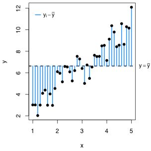 |
(b) 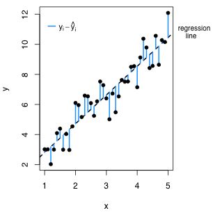 |
| Fig. 3 The two measures of variability that are being compared in the R2 statistic. (a) illustrates the variability about the sample mean and (b) illustrates the variability about the regression line. The amount that the variability has decreased in going from (a) to (b) divided by how much variability there originally was in (a) defines R2. | |
Instead of using average variability, as measured for example by the variance, R2 uses total variability, which is the variability not normalized by sample size. If we let ![]() denote the estimate of the response from the regression equation then R2 can be formulated as follows.
denote the estimate of the response from the regression equation then R2 can be formulated as follows.
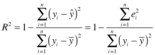
Here n is the number of observations and ei is the residual, i.e., the deviation of the ith observed response value from its estimate on the regression surface. As a demonstration of the formula I calculate the R2 using the formula and compare it to the number that is reported in the regression output.
The statistic labeled "adjusted R-squared" in the output is obtained by modifying the R2 formula so that the two sums of squares terms are replaced by their averages in which unbiased estimates are used for each average. The "adjusted R-squared" can be interpreted as a penalized R2. Adjusted R-squared is not necessarily better than R2 but it has a certain appeal . Ordinary R2 can never decrease when variables are added to a model. It must go up or at worse stay the same. Adjusted R-squared on the other hand can decrease if a newly added variable doesn't decrease the total variability enough. Thus adjusted R-squared can be used in model selection, whereas ordinary R2 is not particularly good for this purpose except in very simple cases.
Categorical predictors pose special problems in regression models. By a categorical predictor I mean a variable that is measured on a nominal (or perhaps ordinal) scale whose values serve only to label the categories.
In experimental data it's common for the response variable to be continuous but for all of the predictors to be categorical. In this situation the various combinations of the values of the categorical predictors are usually referred to as treatments or treatment levels. The categories themselves may be generated artificially by dividing the scale of a continuous variable into discrete categories. Using categories makes it possible to look for gross effects with a limited amount of data. It also avoids the problem of having to determine the proper functional form for the relationship between the response and a continuous predictor. Categorization is also useful in preliminary work where the primary interest is to determine whether a treatment has any effect at all. Typical choices for the discretizing a continuous predictor are:
It's also common for the treatment to be intrinsically categorical. For instance in a competition experiment the "treatment" may be the identity of the species that is introduced as the competitor. In this case the categories would be the different species.
To say analysis of variance is just regression with categorical predictors avoids an obvious question, namely how do you include categorical predictors in a regression model? Categorical predictors are nominal variables, i.e., their values serve merely as labels for categories. Even if the categories happen to be assigned numerical values such as 1, 2, 3, …, those values often don't mean anything. They're just labels. They could just as well be 'a', 'b', 'c', etc.
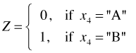
Categorical variables with two levels. Suppose we have a nominal variable x4 with two categories labeled "A" and "B". The usual way to include a categorical variable in a regression model is by creating a set of dummy (indicator) variables. The following single dummy variable could be used to represent the variable x4.
To include the predictor x4 in a regression model we use the variable Z (called now a regressor) instead. This is just a simple linear regression of Y on Z. As usual the regression equation gives the mean of the response variable Y.
![]()
Because Z can take only two values, the regression model returns only two different values for the mean, one for each category of the original variable x4. Table 1 summarizes the relationships between the model predictions and the original categories "A" and "B" by plugging in values for Z in the regression equation.
| Table 1 Regression model for a categorical predictor with two levels |
| x4 | Z | |
| A | 0 | |
| B | 1 |
β0 is the mean for category A. The regression coefficient β1 represents the amount the mean response changes when we switch from category A to category B. As a result a test of H0: β1 = 0 here is a test of whether the means of categories A and B are the same.
Categorical variables with three levels. The true essence of the dummy variable method becomes clear when we consider a nominal variable that has more than two categories. Suppose x5 is a nominal variable with categories "low", "medium", and "high". Converting this predictor into a form suitable for use in a regression model requires the creation of two dummy variables as shown below.
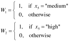
This coding scheme uniquely identifies each of the three categories as follows.
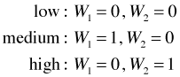
(Observe that the combination W1 = 1 and W2 = 1 is a logical impossibility.) The category we obtain when all of the dummy variables are set equal to zero is called the reference or baseline category. So in the above coding scheme the "low" category is the reference category.
To include the categorical predictor x5 with three categories in a regression model we need to include both of the regressors W1 and W2 in a multiple regression. Once again the regression equation is for the mean of the response variable Y.
![]()
In this case the regression model returns three different values for the mean, one for each category of the original variable x5. Table 2 summarizes the relationships between the categories, dummy variables, and model predictions.
| Table 2 Regression model with a categorical predictor with three levels |
| x5 | W1 | W2 | |
| low | 0 | 0 | |
| medium | 1 | 0 | |
| high | 0 | 1 |
The pattern should now be clear. To include a categorical predictor with k different categories in a regression model, we need to create k – 1 different dummy variables of the kind shown above for k = 3.
With dummy variables we can analyze the relationship between a continuous response and a set of categorical variables (predictors) using standard regression techniques. But the regression approach is not how this problem was formulated initially. The original methodology that was developed to handle a continuous response and categorical predictors is called analysis of variance, or ANOVA. The name seems peculiar. If the goal is to compare treatment means why do we instead analyze variance?
If different treatments have different effects on the response then we expect the treatment means to be very different. But if the treatment means differ by a large amount then the variability among the treatment means will also be large. To quantify what constitutes "large" we need an appropriate standard of comparison. For this we can use the natural variability of the observations making up out study. So, if the average variability of the treatment means is large relative to the average variability of the observations then we can conclude that the treatment effect is important. This is the basis of the F-test that appears in analysis of variance tables.
When we move to other kinds of regression problems later in this course, we'll replace this notion of comparing different sources of variability with comparing the fit of two competing models: one in which we allow the treatment means to differ and a second model in which we constrain the treatment means to all be the same. Still, even in these cases a version of the analysis of variance table is still useful because it's a rather clever way of extracting the maximal amount of information from a regression model in which the response is continuous and the predictors are categorical.
The term treatment is used in analysis of variance to describe the conditions that we impose on an observational unit. These conditions derive from the values of one or more categorical variables. In analysis of variance we refer to a categorical variable as a factor. The values of the categorical variable are called the levels of the factor. An example of a factor would be temperature recorded "low", "medium", and "high". Another example of a factor is temperature recorded 25°C, 28°C, and 32°C. In this case the levels are numeric so we could treat the predictor as continuous. We may still prefer to treat them as just categories for the reasons described previously.
A regression with a continuous response and a single categorical predictor is called a one-way analysis of variance problem. (If the categorical predictor is a factor with just two levels then a one-way ANOVA reduces to an independent two-sample t-test.) A regression with a continuous response and two categorical predictors is called a two-way analysis of variance problem. With two categorical predictors the treatments are created by combining the levels of the two factors in all possible ways and then randomly assigning observations to these combinations. This raises the question, why not just analyze the two-way ANOVA as a one-way ANOVA in which the combined treatments form the levels of a single categorical variable?
One way design. As an illustration suppose we have two factors, denoted H and P, each with two levels, "low" and "high". To make things more concrete suppose this is a greenhouse experiment on plant growth and H is a heat treatment and P is a precipitation treatment. So we combine the two levels of each factor in all possible ways to generate four treatments denoted hp (control, H and P both low), Hp (H high, P low), hP (H low, P high), and HP (H high, P high) as summarized in Table 3.
| Table 3 Two factors treated as a one-way treatment structure |
| Factor | Treatment | |||
| hp | Hp | hP | HP | |
| H (heat) | low | high | low | high |
| P (precipitation) | low | low | high | high |
A factor with four levels gets entered into a regression model as three dummy variables. I choose the control level hp as the reference level.
The regression model is then
![]()
from which we obtain the following estimates of the mean for each treatment.
| Table 4 Cell means for the one-way design of Table 3 |
| Treatment | hp | Hp | hP | HP |
| Mean |
Consequently a test of H0: β1 = 0 tests whether treatment Hp is different from the control, H0: β2 = 0 tests whether hP is different from the control, and H0: β3 = 0 tests whether HP is different from the control.
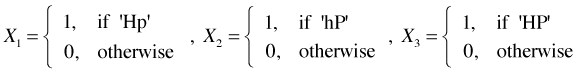
Two-way design. The same experiment can be formulated as a two-way analysis of variance as follows. Create separate dummy variables for the H factor and the P factor as follows.
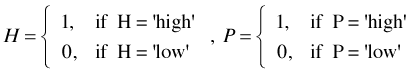
To create the regression model we include both H and P as regressors as well as their product H × P. This yields three regressors just as we had in the one-way formulation of the experiment. Table 5 compares the dummy variable codings for the one-way and two-way formulations of this ANOVA problem.
Table 5 Dummy coding for the four treatments in the two designs |
| Treatment | One-way Design | Two-way Design | ||||
| X1 | X2 | X3 | H | P | H × P | |
| hp | 0 | 0 | 0 | 0 | 0 | 0 |
Hp |
1 | 0 | 0 | 1 | 0 | 0 |
hP |
0 | 1 | 0 | 0 | 1 | 0 |
HP |
0 | 0 | 1 | 1 | 1 | 1 |
Our regression model for the two-way design is the following.
![]()
By plugging in values for H and P in this equation we obtain the following estimates of the mean for each treatment.
| Table 6 Estimated cell means for the two-way design |
| Treatment | hp | Hp | hP | HP |
| Mean |
So, we see that the two-way formulation and the one-way formulation are just different parameterizations of the same experiment, the difference appearing in mean of the HP treatment. The one-way formulation allows us to test whether any of the treatments are different from the control. The two-way formulation allows us to test whether the treatments H and P interact in their effect on the response or instead act in a purely additive manner. The H × P term in the regression model is called an interaction, in this case a two-factor interaction. Fig. 4 illustrates the roles played by the four parameters in the two-way design.
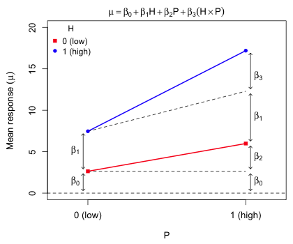 |
| Fig. 4 Depiction of the roles of the regression parameters in the two-way design. The predicted mean response for each treatment is displayed. |
From Fig. 4 we can discern the following.
The attraction of the two-way design is that it allows us to test whether the factors H and P act independently of each other or whether they interact. If factors interact then the effect of one depends on the level of the other. When there's a significant interaction between factors we can't speak of a single effect due to that factor; its effect varies depending on the values of other predictors in the model.
When the two factors H and P interact then there really is no difference between the one-way and two-way formulations of this problem. In both formulations we have four treatment means with no particular relationship between them. Each mean has its own parameter. But, if the factors do not interact then the two-way design is the superior formulation.
In the one-way design we estimate the H effect by comparing treatment Hp to treatment hp (the control). But if H and P do not interact then we can obtain a second estimate of the H effect by comparing treatment HP to treatment hP (P is at its high level for both). We can then average these two estimates of the H effect to obtain a more precise estimate (using more observations). This is exactly what occurs in the two-way design when we drop the interaction term H × P, something we might do if we discover that the interaction is not statistically significant. Without the interaction the four treatment means can all still be different yet we need only three parameters to generate them.
| Jack Weiss Phone: (919) 962-5930 E-Mail: jack_weiss@unc.edu Address: Curriculum for the Environment and Ecology, Box 3275, University of North Carolina, Chapel Hill, 27599 Copyright © 2012 Last Revised--Aug 22, 2012 URL: https://sakai.unc.edu/access/content/group/3d1eb92e-7848-4f55-90c3-7c72a54e7e43/public/docs/lectures/lecture1.htm |