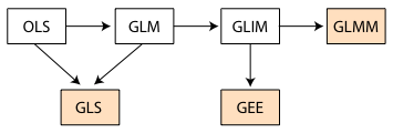
Fig. 1 displays how the various models we've examined in this course relate to each other. I review each model type in turn.
Fig. 1 Flow chart of models considered in this course
This is the classic ordinary regression model in which we have a continuous response y and multiple continuous predictors x1, x2, … , xj . We typically write
Although not essential for estimation but necessary for inference we also assume ![]() , so that the errors are independent and have the same variance.
, so that the errors are independent and have the same variance.
The general linear model is a minor generalization of the ordinary regression model that allows it to include predictors of any sort. In particular we can include categorical predictors in a regression model if we enter them as dummy variables (lecture 2). Historically this realization was important because it meant that many of the classic statistical models, e.g., ANOVA and ANCOVA, are really just instances of regression.
The generalized linear model extends the general linear model to non-normal distributions for the response, in particular, distributions that are members of the exponential family of distributions (normal, binomial, Poisson, etc.). Formally a generalized linear model consists of three parts: (1) a random component, the probability distribution for the response, (2) a systematic component, this is the usual regression model, and (3) a link function g that links the random component to the systematic component. Formally we write the generalized linear model as follows.
where f is a probability distribution characterized by the parameters μ and θ. Unlike the ordinary regression model, parameter estimates of the generalized linear model are obtained using maximum likelihood instead of least squares. This provides us with log-likelihood, deviance, and AIC for model selection.
GLS generalizes both OLS and the GLM to correlated residuals with heterogeneous variances. Formally, we replace the assumption ![]() with the assumption
with the assumption ![]() where
where ![]() . Here V is a diagonal matrix of potentially different (heterogeneous) variance terms and R is a correlation matrix. We considered the case where V had a constant diagonal and R is generated by an ARMA(p, q) process in lecture 17.
. Here V is a diagonal matrix of potentially different (heterogeneous) variance terms and R is a correlation matrix. We considered the case where V had a constant diagonal and R is generated by an ARMA(p, q) process in lecture 17.
Mixed effects models are useful for dealing with correlated hierarchical data, typically where observations come in groups and the observations within a group are more similar to each other than they are to members of other groups. Mixed effects models account for correlation indirectly by modeling observational heterogeneity. They include terms, random effects, that account for the similarities between observations. Formally this is done by extending the generalized linear model as follows. Let i denote the group and j an observation on that group. (For instance i could denote a person and j could denote one of the multiple measurement times on that person in a repeated measures design.)
Here x1, … , xp and z1, … , zq are predictors. Typically, and in all the cases we've considered, the zk are just relabeled members of the set {x1, … , xp}. β0, β1, … , βp are the ordinary regression parameters while u0i, u1i, … , uqi are random effects that vary across groups. We assume the random effects for a single group have a multivariate normal distribution,
and estimate the parameters of Ψ. The random effects from different groups are independent. GLMMs can be estimated using maximum likelihood and thus yield a log-likelihood and AIC. Other choices of estimation, e.g., REML, are also possible and sometimes are the default. The presence of the random effects leads to a subject-specific interpretation of the fixed effect parameters in the model. For models with an identity link the fixed effect parameters also have a marginal (population-average) interpretation.
While mixed effects models are a very general way of handling correlated data they do have their limitations. In particular, they fail to provide a marginal interpretation of the parameters when g is not the identity link. Furthermore the random effects alone can fail to properly account for the correlation in the data. An alternative to mixed effects models in these cases is GEE. GEE estimates the marginal model directly and like GLS requires that the user specify a model for the variance and a model for the correlation. GEE starts with the same estimating equation that is obtained when trying to maximize the log-likelihood of a generalized linear model.
If the right hand side was derived from a log-likelihood, then we can recapture that log-likelihood (up to an additive constant) by antidifferentiating the right hand side. In all other cases we refer to the antiderivative of the right hand side as a quasi-likelihood. In GEE we choose a regression model for μ, typically with a link function, and models for the mean-variance relationship as well as the assumed correlation of the response. These choices together define![]() .
.
The four generalizations of the GLM that we've considered thus far have focused entirely on the random component of the model. With GLIMs we considered probability models other than a normal distribution. We then relaxed the variance model and/or independence assumption of these probability models in different ways with GLS, GLMM, and GEE.
We can also generalize the systematic component of the regression model.
Systematic component: 
What characterizes the systematic component of a generalized linear model is its linearity. The systematic component consists of a sum of predictors (or functions of predictors) that are each multiplied by constant terms, the parameters. We call a regression model linear when it is linear in its parameters.
One way we could generalize things is by abandoning the linear form of the systematic component entirely and writing it as a function of the predictors.
![]()
If we have a parametric form in mind for the function f then we are in the realm of nonlinear regression. This is a well-studied field and there are standard methods for obtaining parameter estimates. We've already seen an example of this in Assignment 4 where you had occasion to use the nls function of R to estimate the nonlinear Arrhenius model. The general problem with nonlinear regression is that there are infinitely many possible nonlinear functions to consider. Unless theoretical considerations suggest a parametric form for f, the situation is rather hopeless.
What about taking a nonparametric approach, using the data to suggest the form of the function f? Consider the case where f is assumed to be a function of two variables, f(x1, x2). Suppose we have n observations whose x1-coordinates adequately cover the range of relevant values of x1 and whose x2-coordinates similarly cover the range of interesting values of x2. Unfortunately when we plot these points in the two-dimensional space of the x1-x2 plane we see that coverage is noticeably sparser. This is referred to as the curse of dimensionality. To get the same coverage with comparable spacing in two dimensions that we had in one dimension requires n2 observations rather than n. (This is actually a bit of an overstatement. Still, the actual number of observations needed is much greater than n and does increase with an increasing power as the number of dimensions increases.) This expansion in the data needed to obtain useful estimates makes full-fledged nonparametric estimation of a nonlinear function f of two or more predictors impractical in most cases.
A compromise approach that avoids the curse of dimensionality is to fit an additive model, a model that takes the following form.
The individual functions, fj, are called partial response functions and they represent the marginal relationship between the mean response and an individual predictor. Each fj is a function of one variable. In the additive model ![]() replaces the parametric terms
replaces the parametric terms![]() . The fj are completely unspecified and do not depend on any parameters. For this reason the fj are also called nonparametric regression estimators or "smoothers". In the R mgcv package that fits additive models an additive model with three predictors is written as follows: y ~ s(x1) + s(x2) + s(x3) where the s() notation is used to represent a generic smoother.
. The fj are completely unspecified and do not depend on any parameters. For this reason the fj are also called nonparametric regression estimators or "smoothers". In the R mgcv package that fits additive models an additive model with three predictors is written as follows: y ~ s(x1) + s(x2) + s(x3) where the s() notation is used to represent a generic smoother.
Working with GAMs requires a profound adjustment in the way we view a regression model.
GAMs can be treated as a full-fledged approach to modeling, Zuur et al. (2007) and Zuur et al. (2009) are strong proponents of this viewpoint, or as a way of suggesting possible transformations of the predictors that can then be used in parametric regression models. Packages that fit GAMs are flexible and allow users to treat some terms in the regression model parametrically and other terms nonparametrically. For instance, factor variables, which can't be smoothed, need to be entered into the model parametrically. An additive model that contains both parametric and nonparametric terms (smoothers) is called a semiparametric regression model.
To better understand the additive model we start by exploring how the individual partial response functions, the fj, are obtained in practice. Because the overall model is additive we can restrict ourselves to the one variable nonparametric regression problem, ![]() . Given a scatter plot of y versus x we wish to find a function f that best approximates the relationship between the two variables. Two popular ways of obtaining f are local polynomial regression (lowess) and spline regression. We consider each approach in turn.
. Given a scatter plot of y versus x we wish to find a function f that best approximates the relationship between the two variables. Two popular ways of obtaining f are local polynomial regression (lowess) and spline regression. We consider each approach in turn.
Local polynomial regression is more commonly known as lowess or loess. Lowess is an acronym for LOcally WEighted Scatterplot Smoother. We briefly considered lowess in lecture 11. Lowess is based on the following five ideas.
We consider each of these ideas in turn.
Binning turns a continuous variable into a categorical one. It recognizes that the x-values near a particular x0 provide us with additional information about f(x0). In binning we use the x-variable to construct the bins by dividing the x-axis into intervals that in turn define categories for the corresponding values of the y-variable. In the simplest version of binning we calculate the mean of the y-variables in each of the bins. The mean of the y-variables is assigned to the x-coordinate at the midpoint of each bin. To obtain f we connect these points with line segments after sorting the means by their corresponding x-variable.
The main difficulty with binning is in choosing the bins. If the bins are large then the predicted y-value will differ quite a bit from the individual y-values (high bias) although it will be stable under repeated sampling (low variance). If the bins are small then we approximate the individual y-values well (low bias) but the estimates will vary markedly with repeated sampling (high variance). The variance-bias trade-off suggests we need a better approach.
We can obtain an estimate of y at each of the unique values of x if we are willing to reuse data. With this in mind local averaging replaces the fixed bins with a moving window. Consider a specific value of x, denote it x0. We start with a window centered at x0, now referred to as the focal value. For all the observations within the window we average their values of the y-variable to obtain the estimate f(x0). The process then moves to the next unique x-value, x1, and the process is repeated to obtain the estimate f(x1).
The different windows overlap so the data get reused many times. In choosing the windows we can specify their width (now called the bandwidth) or we can instead require that each window contains a specified fraction of the data, referred to as the span. For instance if there are n observations and we wish each window to contain m of them, we choose a variable bandwidth so that the span ![]() is the same for each window. As with binning in the end we obtain a graph of f(x) by connecting the individual means after first sorting them by their corresponding x-variable.
is the same for each window. As with binning in the end we obtain a graph of f(x) by connecting the individual means after first sorting them by their corresponding x-variable.
Local averaging typically yields a curve that is rather choppy as observations come and go. Furthermore while points near x0 are indeed informative about f(x0), they are not equally informative. We can get a smoother curve if we replace local averaging with locally weighted averaging, also known as kernel estimation. A kernel function is one that weights observations that are close to the focal value more heavily than observations that are far away. There are standard choices for the kernel functions a topic we'll explore next time.
| Jack Weiss Phone: (919) 962-5930 E-Mail: jack_weiss@unc.edu Address: Curriculum for the Environment and Ecology, Box 3275, University of North Carolina, Chapel Hill, 27599 Copyright © 2012 Last Revised--March 13, 2012 URL: https://sakai.unc.edu/access/content/group/2842013b-58f5-4453-aa8d-3e01bacbfc3d/public/Ecol562_Spring2012/docs/lectures/lecture24.htm |