#Gleason Model
The estimated model is μ = –171.03 + 109.44 × log(area), where μ is the mean of species richness.
#log-Arrhenius Model
The estimated model is μ = 3.84 + 0.33 × log(area), where μ is the mean of log(species richness). Alternatively we can interpret exp(μ) as either the median or the geometric mean of species richness (see lecture 7).
#Arrhenius model
I exponentiate the estimates obtained from the log-Arrhenius model for use as initial estimates to the nls function for the Arrhenius model.
The estimated model is μ = 83.48 × area0.26, where μ is the mean of species richness.
#Poisson model
The estimated model is log μ = 4.19 + 0.28 × log(area), where μ is the mean of species richness.
#Negative binomial model
The estimated model is log μ = 3.97 + 0.32 × log(area), where μ is the mean of species richness.
Summarizing we have the following results. μ denotes mean richness except in the log-Arrhenius model where it denotes mean log richness.
| Model | Fitted equation |
| Gleason | μ = –171.03 + 109.44 × log(area) |
| log-Arrhenius | μ(log richness) = 3.84 + 0.33 × log(area) |
| Arrhenius | μ = 83.48 × area0.26 |
| Poisson | log μ = 4.19 + 0.28 × log(area) |
| negative binomial | log μ = 3.97 + 0.32 × log(area) |
The log-Arrhenius model, because it models the log of species richness, stands alone and I plot it by itself. The Gleason model and Arrhenius model are also graphically incompatible. But the Poisson model and negative binomial model are of the same form. They can be plotted together with the Gleason model, or together with the Arrhenius model, as I show below.
#Log-Arrhenius model
#Arrhenius model
(a) 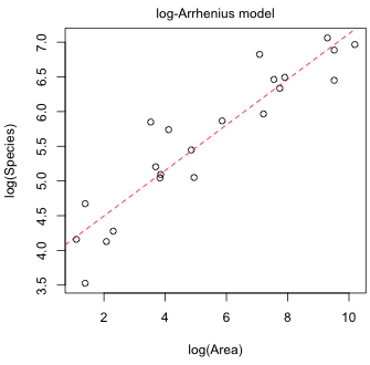 |
(b) 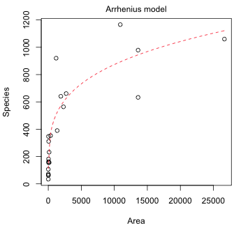 |
| Fig. 1 Mean log(richness) and mean richness predicted by the log-Arrhenius and Arrhenius models, respectively. | |
#Gleason, Poisson, and negative binomial models
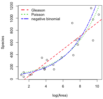
Fig. 2 Mean richness as a function of log area as predicted by the Gleason, Poisson, and negative binomial models
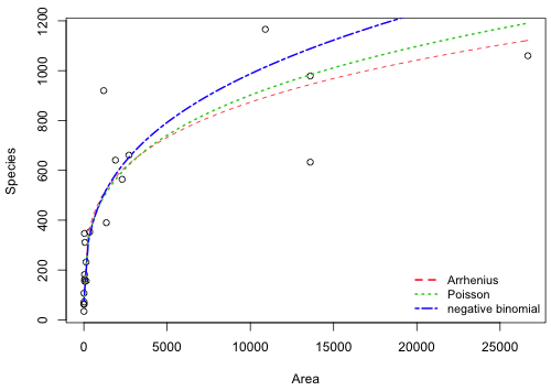
As explained above the Arrhenius, negative binomial, and Poisson models can be grouped together.
 |
|
| Fig. 3 Mean richness as a function of area as predicted by the Arrhenius, Poisson, and negative binomial models | |
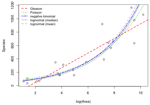
The log-Arrhenius model can be added to the negative binomial, Poisson, and Gleason models either as the median or the mean, which are not the same here. Exponentiating the lognormal model does not return the mean, but instead returns the median on the raw scale. The lognormal distribution is typically positively skewed so that the median and mean are very different. The mean of the lognormal distribution can be expressed in terms of μ and σ2, the mean and variance of the log-transformed variables.
 |
|
| Fig. 4 Modeled richness as a function of log(area) as predicted by the Gleason, Poisson, negative binomial, and lognormal models | |
The log-likelihood for the log-Arrhenius model needs to be calculated separately since the response is log-transformed in this model. We have two versions of this function from lecture 11 which here yield barely different results. There is no additive constant in our model so I set k = 0 when using the functions.
I create a list of model names, string together the log-likelihoods, list the number of estimated parameters in each model, and calculate the AIC values. Three parameters are estimated in each model (two regression parameters and an auxiliary parameter—the variance for normal models and the dispersion for the negative binomial), except the Poisson model in which only two parameters were estimated.
From the reported AIC values only the log-Arrhenius and negative binomial models are reasonable models for these data.
It's worth reflecting on the fact that in Fig. 2, the graphs of the worst model (the Poisson) and one of the best models (negative binomial) are virtually identical. In a least squares sense these two models would be found to be nearly indistinguishable, but of course we didn't use least squares to fit these models. We used maximum likelihood. In maximum likelihood we're not evaluating fit by how close the mean trajectory comes to the observations. Instead we're trying to maximize the probability of obtaining the observed data. Thus when we compare models using log-likelihood or AIC we're evaluating probability generating mechanisms. From the log-likelihood (or the AIC) reported in the above table we would conclude that it is very unlikely that a Poisson model generated these data. It is far more likely for a negative binomial model to have generated these data.
| Jack Weiss Phone: (919) 962-5930 E-Mail: jack_weiss@unc.edu Address: Curriculum for the Environment and Ecology, Box 3275, University of North Carolina, Chapel Hill, 27599 Copyright © 2012 Last Revised--February 16, 2012 URL: https://sakai.unc.edu/access/content/group/2842013b-58f5-4453-aa8d-3e01bacbfc3d/public/Ecol562_Spring2012/docs/solutions/assign4.htm |