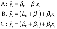
(a) 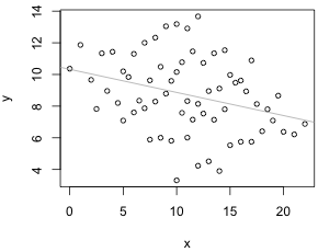
(b) 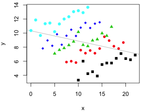
Consider the artificial data set shown in Fig. 1. We plot y versus x and superimpose the estimated regression line. The response variable y appears to decrease as a function of the predictor x (Fig. 1a).
(a) |
(b) |
| Fig. 1 (a) Scatter plot of y versus x suggesting a linear relationship with regression line superimposed. (b) It turns out that the observations can be classified into five groups as denoted by the colored symbols. | |
Indeed the statistical output from the fitted regression model indicates the relationship is statistically significant.
Analysis of Variance Table Response: y |
It turns out that these observations divide into groups and within these groups the relationship between y and x appears to be quite different, positive rather than negative (Fig. 1b). In practice the groups could be different taxa or the different treatment groups in an experiment. Fig 2a shows the results of estimating the regression relationship between y and x separately for each group.
(a) 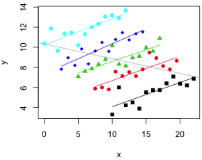 |
(b) 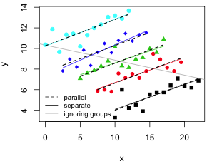 |
| Fig. 2 (a) Separate regression lines fit to each group. (b) Separate regression lines fit to each group (interaction model) along with parallel regression lines fit to the groups (no interaction model). | |
Let the groups be denoted by the categorical variable z. Fig 2a suggests that when we account for z our interpretation of the relationship between y and x changes.
Formally Fig 2a is not a demonstration of confounding because we've done too much. In Fig. 2a we've allowed the relationship between y and x to be different for each level of z. Therefore Fig 2a is an example of what's called an interaction model. Confounding is a far simpler idea. To determine if z is a cofounder we just include z in the model to see if our interpretation of the relationship between y and x changes in a substantive fashion. The model we obtain is called an additive model and when z is a categorical variable it corresponds to a set of parallel lines (Fig. 2b).
For the additive model to make sense we should have first rejected an interaction model. In Fig. 2b where both the interaction model (separate lines) and the no interaction model (parallel lines) are compared, it's pretty clear that there is very little difference between them. The two sets of lines look about the same. A formal statistical test (Table 1) demonstrates that the interaction terms are not statistically significant.
Table 1 Testing for an interaction |
lm(formula = y ~ x + z + x:z, data = mydat) Response: y |
Having rejected the interaction model we can proceed to check for confounding. For that we compare the coefficient of x in a model that contains z with the coefficient of x in a model that omits z. The output from R for these two models is shown in Table 2 where the coefficient of x is highlighted in yellow. The output confirms what we've already concluded from Fig. 2. The relationship between y and x changes from negative to positive when z is included in the model. Because there is no significant interaction between x and z it is legitimate to call z a confounder.
Table 2 Checking for confounding |
Model without z lm(formula = y ~ x, data = mydat) Coefficients: |
Model containing z lm(formula = y ~ x + z, data = mydat) Coefficients: |
Interactions are specified in regression models by including terms that are the products of the individual predictors. Suppose we have two predictors x and z where x is the variable of primary interest and z is a control variable. A model that includes x and z as predictors of a response y is referred to as an additive model.
![]()
A regression model with a single continuous predictor x represents a line in two-dimensional space. The above regression model with a continuous x and a continuous z represents a plane in 3-dimensional space. (If z is categorical then this model represents a set of parallel lines, one for each category of z. See below.)
An interaction model must includes all of the terms of the additive model in addition to the product of the variables x and z.
![]()
To understand what this equation represents I group the terms that involve x together.
Unlike the additive model, the coefficient of x is no longer constant. It changes depending on the value of z. This is the definition of interaction. The effect of one variable depends on the value we assign to another.
The interaction model where both x and z are continuous can be represented geometrically as a curved surface in 3-dimensional space (as compared to a plane for the additive model). If on the other hand x is continuous but z is categorical then the interaction model represents a set of non-parallel lines in two-space (as compared to a set of parallel lines for the additive model).
Categorical predictors pose special problems in regression models. By a categorical predictor I mean a variable that is measured on a nominal (or perhaps ordinal) scale whose values serve only to label the categories. The categories of a categorical variable are referred to as its levels.
The common situation with experimental data is that the response variable is continuous but most if not all of the predictors are categorical. In this situation the categorical predictors are often referred to as treatments. The treatments may have been generated artificially by dividing the scale of a continuous variable into discrete categories. Using categories we can get by with fewer observations and avoid the need to determine the exact functional relationship between the response and the treatment (as would be necessary if it were treated as continuous). Categorization is helpful in preliminary work where the main goal is to determine if a treatment has any effect at all.
Typical choices for the categories in experiments are:
It's also common for the treatment to be intrinsically categorical. For instance in a competition experiment the "treatment" might be the identity of the species that is introduced as the competitor. In this case the categories would be the different species.
The analysis of the relationship between a continuous response and a set of categorical variables (predictors) is easily handled by standard regression techniques. Historically the methodology developed to handle this situation was called analysis of variance, or ANOVA. In its modern implementation ANOVA is just regression although the usual way it is presented may not look like it. As an organizational tool ANOVA turns out to be a very clever way of extracting the maximal amount of information from a regression problem in which the response is continuous and the predictors are categorical.
If the primary focus is still on the categorical predictors but we've also included one or more continuous predictors in the model to act as control variables, the model is referred to as an analysis of covariance (ANCOVA) model. The terms ANOVA and ANCOVA although a bit anachronistic are still useful in identifying the primary focus of an analysis.
To say that analysis of variance is just regression with categorical predictors avoids the obvious question: how do you include categorical predictors in a regression model? Categorical predictors are nominal variables, so their values serve merely as labels for the categories. Even if the categories happen to be assigned numerical values such as 1, 2, 3, …, those values don't mean anything. They're just labels. They could just as well be 'a', 'b', 'c', etc.
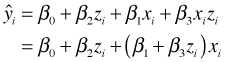
Suppose you were to ignore this fact and treat the categories as numerical. Let the variable z have three categories, A, B, and C, that we choose to encode as 1, 2, and 3. We then fit the regression model
![]()
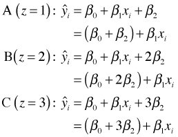
This corresponds to three different equations, one for each value of z (Fig. 3).
 |
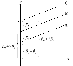 |
| Fig. 3 The results of assigning numerical values to the categories of a categorical predictor | |
Fig. 3 reveals that this choice of coding has place some unnatural constraints on the lines we obtain. The effect of z is to change the location of the intercepts of the three lines. While no constraint has been placed on the intercepts of lines A and B, line C is forced to be the same distance from line B as line B is from line A. If we were to carry out a test of H0: β2 = 0 in this model it would be a test of whether the lines of all three groups have the same intercept (and hence the three lines coincide). There is no way with this choice of coding to test whether the intercepts of lines B and C are the same, but are different from line A.
The most common way to include a categorical predictor in a regression model is with a dummy (indicator) coding scheme. In general, a categorical predictor with m categories requires that we include m – 1 dummy variables. One of the m categories is chosen as the reference category while the rest of the categories are indicated by the individual dummy variables.
For the example we've been considering, a categorical variable z with three categories A, B, and C, a dummy coding scheme in which A serves as the reference category is the following.
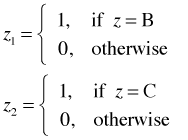
This coding scheme uniquely identifies the three categories as follows.
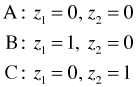
Observe that the combination z1 = 1 and z2 = 1 is a logical impossibility here. The reference or baseline category is obtained when all of the dummy variables are set equal to zero.
To distinguish the concept of a predictor from the terms that are used to represent it in a regression model, we refer to the latter as regressors. So to include the 3-category predictor z in a regression model we need to include two dummy regressors z1 and z2. An additive regression model that uses x and z to predict the value of y is the following.
![]()
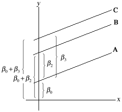
This regression model corresponds to three different equations, one for each of the categories of the original variable z. Table 3 summarizes the relationships between the categories, dummy variables, and model predictions. The three equations represent three lines with different intercepts but the same slope.
| Table 3 Regression model with a categorical predictor with three levels |
| z | z1 | z2 | |
| A | 0 | 0 | 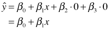 |
| B | 1 | 0 | 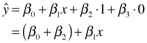 |
| C | 0 | 1 | 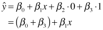 |
Fig. 4 shows the corresponding lines that we obtain. Unlike the situation in Fig. 3, now the intercept of each line is unconstrained. Furthermore testing whether the lines are different is easy. H0: β2 = 0 tests whether lines A and B coincide. H0: β3 = 0 tests whether lines A and C coincide, and H0: β2 = β3 tests whether lines B and C coincide.
 |
 |
| Fig. 4 The effect of using dummy variables to represent the categories of a categorical predictor in a regression model | |
To construct the interaction of two continuous variables we take their product. When one of the variables is categorical we instead take the product of the corresponding regressors. So in our example involving the predictors x and z where z is represented by the dummy variables z1 and z2, the interaction model would take the following form.
![]()
As before the regression model corresponds to three different equations, one for each category of the original variable z. Table 4 summarizes the relationships between the categories, dummy variables, and model predictions. By including interactions between a continuous predictor and dummy regressors, we allow the line for each group to have a different slope (as well as a different intercept).
| Table 3 Interaction model with a categorical predictor with three levels |
| z | z1 | z2 | |
| A | 0 | 0 | 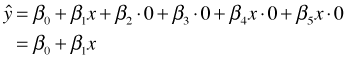 |
| B | 1 | 0 | 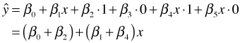 |
| C | 0 | 1 | 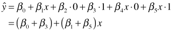 |
To test whether all three lines have the same slope we would need to test the hypothesis H0: β4 = β5= 0. If we fail to reject this hypothesis then we're reduced to the additive model discussed above.
The R code used to generate Figs. 1 and 2 appears here.
| Jack Weiss Phone: (919) 962-5930 E-Mail: jack_weiss@unc.edu Address: Curriculum of the Environment and Ecology, Box 3275, University of North Carolina, Chapel Hill, 27599 Copyright © 2012 Last Revised--Jan 12, 2012 URL: https://sakai.unc.edu/access/content/group/2842013b-58f5-4453-aa8d-3e01bacbfc3d/public/Ecol562_Spring2012/docs/lectures/lecture2.htm |