Assignment 3— Solution

Question 1

I read in the data, convert Density to a factor, and fit the two-factor analysis of variance model with Eggs as the response and Season, Density, and their interaction as predictors as in Assignment 1.

I next obtain the data frame of means and 95% confidence intervals that we constructed in Assignment 2. The easiest way to obtain the means is to trick R into giving them to us by fitting the following model in which we remove the intercept and include only the interaction term. Alternatively you can use the predict function as was shown in the Assignment 2 solutions.

The only new part of this problem is to obtain the difference-adjusted confidence levels so that we can make pairwise comparisons between the means. For that we need the ci.func function that was provided you in lecture 5.

To use this function we need the variance covariance matrix of the means. Using the shortcut approach above I can obtain it by applying vcov to my model of cell means.

If instead we use the original model with the effect estimates then we have to obtain the variance-covariance matrix by matrix multiplication.

Using either approach we get the same answer. We need a confidence level of 85% for all the pairwise comparisons.

I add 85% confidence intervals to data frame of means.

I now just repeat the graph from Question 3 of Assignment 2. The only change is that I add error bars corresponding to the 85% confidence intervals. The changes are highlighted below.

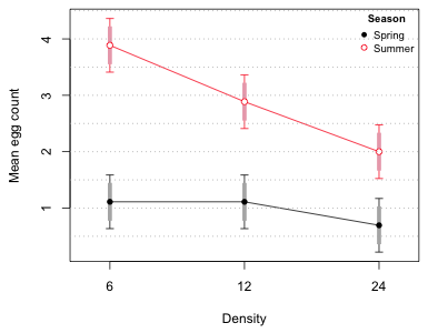
Fig. 1  Interaction plot with difference-adjusted confidence intervals

Based on the display we see that none of the mean egg counts at different densities in Spring are significantly differnet from each other. But in summer the mean egg counts at the three densities are all different from each other. Of course we already knew the spring means and summer means were different because the 95% confidence intervals didn't overlap.

Question 2

Part a

From the description we should probably treat this as a randomized block design in which location defines the block and species is the treatment. Because we have multiple individuals of the same species at each location we are able to test for a treatment × block interaction.

Response: diam
                         Df Sum Sq Mean Sq F value   Pr(>F)  
factor(location)          3  68.05  22.683  1.2726 0.294392  
species                   2 284.93 142.467  7.9925 0.001009 **
factor(location):species  6 157.60  26.267  1.4736 0.207343  
Residuals                48 855.60  17.825                   
---
Signif. codes:  0 ‘***’ 0.001 ‘**’ 0.01 ‘*’ 0.05 ‘.’ 0.1 ‘ ’ 1

The interaction is not significant so we can fit the standard randomized block design model.

Response: diam
                 Df  Sum Sq Mean Sq F value   Pr(>F)  
factor(location)  3   68.05  22.683  1.2089 0.315317  
species           2  284.93 142.467  7.5930 0.001242 **
Residuals        54 1013.20  18.763                   
---
Signif. codes:  0 ‘***’ 0.001 ‘**’ 0.01 ‘*’ 0.05 ‘.’ 0.1 ‘ ’ 1

We find the species effect is significant. To see which species differ we can examine the summary table.

So, species A and B are significantly different but species A and C are not. Because the mean diameter of species B exceeds A whereas the mean diameter of species C is less than A, it's pretty clear that species B is also different from species C. To test this formally we can refit the model choosing a different species as the reference group. I choose species B as the reference group

Now we see that species C is significantly different from species B also.

Note: In a randomized block design one generally does not test for a block effect. In most situations the reported F-statistic for the block effect does not truly have an F-distribution so the reported p-value is incorrect. Even when the F-distribution of the statistic holds we are forced to make the additional assumption that the individuals were randomly assigned to blocks, which is usually not the case. The larger point is that blocks are a part of the design structure of the experiment; they are not part of the treatment structure. Thus blocks should be retained regardless of what the significance tests suggest. For further discussion on this point see lecture 7.

Part b

In the fixed effects version of the randomized block design while we can estimate species differences but we can only estimate the mean diameters of individual species for specific blocks. To get around this we can treat block as a random effect in which case the regression model is formulated for the average individual of each species. In the mixed effects model the block effects (random effects) represent deviations from that average.

Method 1: Using the nlme package plus hand calculations

We can calculate the confidence intervals for the means by hand as follows. I first fit the model using lme.

The degrees of freedom we need for the t-distribution are contained in the fixDF component of the model in a term labeled X.

$terms
(Intercept)     species
         54          54

attr(,"assign")
attr(,"assign")$`(Intercept)`
[1] 1

attr(,"assign")$species
[1] 2 3

attr(,"varFixFact")
          [,1]       [,2]     [,3]
[1,] 0.6148623  0.0000000  0.00000
[2,] 0.3954213 -1.1862640  0.00000
[3,] 0.6848898 -0.6848898 -1.36978

Next I construct a vector that can be used to construct the terms of the regression model.

To get the contrast matrix I sapply this function on a vector of species names. I then use the contrast matrix to obtain the means and standard errors of the means in the usual fashion.

Method 2: Using the nlme package and the intervals function

If we fit the random effects model without the intercept term, lme returns the mean diameter for each species. We can then obtain 95% confidence intervals for the treatment means by using the intervals function.

 Fixed effects:
            lower  est.    upper
speciesA 17.84163 19.85 21.85837
speciesB 21.04163 23.05 25.05837
speciesC 15.74163 17.75 19.75837
attr(,"label")
[1] "Fixed effects:"

Method 3: Using the lmer package and obtaining means via MCMC sampling

Using the lme4 package we can generate Bayesian samples from the posterior distributions of the parameters in the model. These can then be used to construct the means and their confidence (credible) intervals.

Obtain 10,000 samples from the posterior distribution of each parameter.

To obtain the posterior distributions of the means we just have to construct the means from their effect estimates. The mean of species A is the intercept in the model which is column 1, the mean of species B is the intercept plus the species B effect (column 1 plus column 2), and the mean of species C is the intercept plus the species C effect (column 1 plus column 3).

Finally I obtain the .025 and .975 quantiles of each column of new.dat to obtain the 95% percentile credible intervals for the means. For a point estimate of the mean I can take either the mean or the median of the individual posterior distributions.

Course Home Page