The data set alligators.csv comes from Agresti (2002) but it is used in many other textbooks as an example of multinomial data. It's from a study by the Florida Game and Fresh Water Fish Commission of the types of food that alligators choose to eat in the wild. A sample of 219 alligators was obtained from four Florida lakes. For each alligator the primary food type (by volume) was determined from the animal's stomach contents. Food type categories used were birds, fish, invertebrates, reptiles, and other. The invertebrates were primarily apple snails, aquatic insects, and crayfish. The reptiles were primarily turtles although one stomach contained the tags of 23 baby alligators that had been released in the lake the previous year. The "other" category included amphibians, mammals, plant material, stones, and other debris. In addition to lake, the gender of the animal was noted and its size was recorded as either less than or equal to 2.3 meters or greater than 2.3 meters. The purpose of categorizing size in this way was to distinguish subadults from adults.
Each line of the data file is the record of a single alligator listing the predominant food type in its stomach as well as its size, gender, and the lake where it was captured. This is the multinomial equivalent of binary data. Without additional information an appropriate probability could be either multinomial or Poisson.
As we saw in lecture 38, the distinction between Poisson or multinomial doesn't really matter here because by conditioning on the sample size a Poisson distribution becomes a multinomial distribution.
I cross-tabulate the observations by food type, lake, size, and gender to see the distribution of observations across the categories.
We see that the data are rather sparse. Many of the possible combinations of food type, size, gender, and lake were not observed.
The multinom function in the nnet package can be used to fit baseline category multinomial logit models. The multinomial variable is entered as the response and predictors are included using the usual formula notation of R. I start by fitting a null model, a multinomial model with no predictors. I then follow it up with separate models that include each of the the three predictors lake, size, and gender individually.
The anova function applied to two nested multinom models carries out a likelihood ratio test.
Response: food
Model Resid. df Resid. Dev Test Df LR stat. Pr(Chi)
1 1 872 604.3629
2 gender 868 602.2589 1 vs 2 4 2.104069 0.7166248
From the output above we see that the effect of gender is not statistically significant. Nested and non-nested models can be compared using AIC.
The lake-only model ranks best followed by the size model. Including both lake and size in the model leads to a further improvement in the AIC.
Furthermore both terms are statistically significant in the presence of the other.
Response: food
Model Resid. df Resid. Dev Test Df LR stat. Pr(Chi)
1 lake 860 561.1677
2 lake + size 856 540.0803 1 vs 2 4 21.08741 0.0003042795
Response: food
Model Resid. df Resid. Dev Test Df LR stat. Pr(Chi)
1 size 868 589.2134
2 lake + size 856 540.0803 1 vs 2 12 49.13308 1.982524e-06
If we try to add gender to this model we find that it's not needed.
Response: food
Model Resid. df Resid. Dev Test Df LR stat. Pr(Chi)
1 lake + size 856 540.0803
2 lake + size + gender 852 537.8655 1 vs 2 4 2.214796 0.6963214
The summary function applied to the model yields the coefficient estimates and their standard errors.
Coefficients:
(Intercept) lakehancock lakeoklawaha laketrafford size>2.3
fish 2.723723 -0.6950850 0.6531363 -1.08768971 -0.6306971
invert 2.632914 -2.3534487 1.5903438 0.03428501 -2.0888952
other 1.150998 0.1311222 0.6587950 0.42869526 -0.9622560
rep -0.942082 0.5476742 3.1120046 1.84756421 -0.2794163
Std. Errors:
(Intercept) lakehancock lakeoklawaha laketrafford size>2.3
fish 0.7103906 0.7812574 1.202038 0.8416676 0.6424797
invert 0.7266419 0.9337072 1.227725 0.8631499 0.6939064
other 0.8059565 0.8919633 1.368529 0.9382990 0.7127082
rep 1.2411890 1.3715034 1.585983 1.3173183 0.8062283
Residual Deviance: 540.0803
AIC: 580.0803
Because the multinomial response has five categories four sets of coefficient estimates are reported. The category "bird" being first alphabetically was chosen as the reference group for food.
The four rows of the coefficient table correspond to separate models for the log odds (fish vs bird), the log odds (invert vs bird), the log odds (other vs bird), and the log odds (reptile vs bird). The reference group for lake is Lake George and the reference group for size is subadult. In the log odds (fish vs bird) equation we see that the log odds for subadult alligators (size < 2.3) in Lake George is 2.72 (the value of the intercept). This log odds decreases in Lake Hancock and Lake Trafford, but increases in Lake Oklawaha. Because the model is additive in lake and size, the log odds of fish vs bird is decreased by 0.63 for adults relative to subadults in each of the four lakes.
To obtain a formal statistical test of the lake and size effects for each of food log odds models we can divide the coefficients by their standard errors to obtain a Wald test.
Coefficients larger than two in magnitude are statistically significant. Alternatively we can calculate a two-tailed p-value ourselves.
From the output we determine that the log odds of fish or invertebrates relative to birds is statistically significant (greater than zero) in Lake George. The other two log odds are not significantly different from zero in Lake George. The log odds of invertebrates to birds is significantly lower in Lake Hancock than it is in Lake George, while the log odds of reptiles relative to birds is significantly higher in Lake Oklawaha than in Lake George. The only significant size effect is in the log odds of invertebrates to birds with higher odds being favored for subadults than for adults. The statements about log odds ratios can be made more interpretable by exponentiating the log odds coefficients to obtain odds ratios.
Thus we see that the odds of invertebrates to birds being the predominant food type is ten times higher in Lake George than in Lake Hancock, the odds of reptiles to birds being the predominant food type is 22 times higher in Lake Oklawaha than in Lake George, and the odds of invertebrates to birds being the predominant food type is 8 times higher in subadults than in adults.
In the alligator data set each observation is a single realization of a multinomial random variable. We can also fit models to grouped multinomial data, which is the way multinomial data are commonly recorded. To reorganize the current data set in this way, I make a table of food by lake by size and by gender and reorganize it as a data frame, adding the appropriate variable names to the columns.
To fit a multinomial model to data organized in this fashion we have to include the variable that records the counts in the weights argument of multinom. The AIC and log-likelihood we obtain match those obtained with the ungrouped data set.
The vglm function of the VGAM package (which we'll use below for ordinal regression models) can also be used to fit the baseline category multinomial logit model. For this we need to specify multinomial in the family argument with the desired level to use as the reference level. To fit model fit4 using VGAM we would proceed as follows.
The results are virtually identical to what we obtained with the multinom function.
As was explained in lecture 38, multinomial models can be fit as Poisson models by fixing the margin totals. In formulating the model this means including a large number of auxiliary variables. For instance, the null multinomial model fit0 could be fit with a weights argument as follows.
Here is how you would fit the same model using a Poisson distribution.
The count variable is the response and all the predictors and the response are entered as main effects. In addition all of the interactions between the predictors are included.
The logic behind this is as follows. There are 80 rows in the weighted version of the data set, one row per food type. If we divide by the number of food types (5) we get 16, the total number of multinomial observations. We need to constrain these 16 totals in order to get a multinomial distribution. Because these 16 observations are uniquely defined by their combined levels of gender, size, and lake, we can constrain the 16 marginal totals by including gender*size*lake in the model.
We also need to constrain the marginal totals for the five food categories, so we also include food in the model. Thus lake*size*gender + food must be included in every Poisson model we fit in order to match the results from the multinomial regression model.
Whatever variable or combination of variables uniquely identifies the multinomial totals in a data set is what we need to include in the Poisson model. If there had been an ID variable numbered 1 through 16 that identified the 16 multinomial observations, we could have used that as the predictor instead of gender*size*lake. The models we would get are the same, just parameterized differently.
To test the effect of a predictor on food type in the Poisson model we have to add it to the null model as an interaction with food.
If we compare the null Poisson model with the gender Poisson model using a likelihood ratio test we get the same test statistic that we obtained with the multinomial models.
Response: food
Model Resid. df Resid. Dev Test Df LR stat. Pr(Chi)
1 1 872 604.3629
2 gender 868 602.2589 1 vs 2 4 2.104069 0.7166248
Our final multinomial model was one that included lake and size as predictors. To fit this as a Poisson model we need to add food:size and food:lake to the null model.
glm4 <- glm(Freq~lake*size*gender + food + food:lake + food:size, data=alli.dat, family=poisson)
When multinomial data come grouped it is possible to test the fit of the final model by comparing it to a model in which each observation is assigned its own parameter. This is called the saturated model. We have artificially grouped the multinomial data by cross-classifying observations by lake, gender, and size. This yields a distribution of food types for each combination of lake, gender, and size. As was explained above, when the data are organized in this way we have 80 rows of data but only 16 different multinomial observations. Because there are four lakes, two genders, and two sizes, the saturated model requires 4 × 2 × 2 = 16 parameters per logit for a total of 64 parameters. We enter lake*size*gender as the predictor because the 16 multinomial observations are uniquely identified by the 16 different combinations of lake, size, and gender. Again, any variable that uniquely identifies these 16 multinomial observations could be used instead to fit the saturated model.
Alternatively we could have used the ID variable created above to to fit a separate model to each multinomial observation.
In the Poisson version the marginal constraints are enforced by entering lake*size*gender + food. To estimate the same effects shown in the saturated multinomial model fit.S we need to interact food with all the individual terms shown there: lake*size*gender. So we would have to write the following.
We can obtain all these terms with the following simpler expression.
Freq ~ lake*size*gender*food
The total number of estimated parameters is 80, one for each observed count. With the Poisson version we can check to see that we've done things correctly because the residual deviance of the saturated model will be zero and the number of estimated coefficients is equal to the number of observations.
Alternatively we could have used the ID variable created above to identify the multinomial observations and fit the saturated model as follows.
A formal goodness of fit test uses a likelihood ratio test to compare the model of interest against the saturated model. If the p-value is significant then we have a significant lack of fit.
Model 1: Freq ~ lake * size * gender + food + food:lake + food:size
Model 2: Freq ~ lake * size * gender * food
Resid. Df Resid. Dev Df Deviance Pr(>Chi)
1 44 52.478
2 0 0.000 44 52.478 0.1784
From the output it would appear that we don't have evidence of lack of fit.
This goodness of fit test based on residual deviance is identical to the G-test of Sokal and Rohlf (2012), which in turn is asymptotically equivalent to the Pearson chi-squared goodness of fit test. If Oi is the observed count and Ei is the expected count predicted by the model, then the G-test and Pearson test are the following.
G-test:
Pearson test: 
Both test statistics have an asymptotic chi-squared distribution with n – p – 1 degrees of freedom where p is the number of estimated parameters in the model. Both of these tests have restrictions on how small the expected counts can be in order for the chi-squared distribution to still hold. A seat of the pants rule is that no more than 20% of the expected cell counts should be less than 5. We can readily check this by obtaining the predicted counts from the Poisson model. (I exponentiate the predictions because the Poisson model uses a log link. I could have used the fitted function instead, which inverts the link function after obtaining the predictions.)
So we see that 75% of the expected counts are less than 5. The chi-squared distribution of the goodness of fit test is questionable here, so we should not trust the conclusion of the test that the fit is adequate.
When the theoretical distribution of a test statistic is suspect we can turn to Monte Carlo methods. The idea behind a Monte Carlo test is simple. Since we don't know what the theoretical distribution of our test statistic should be, we generate an empirical approximation to the distribution instead. For the current problem that means using our fitted multinomial model to generate new data. Treating the generated data as a new set of observations we carry out the G-test to obtain the G statistic for the simulated data. We then do this repeatedly to obtain a distribution of G-statistics for data that we know are consistent with our model (because the model generated them). We then check to see if the G-statistic obtained using the actual data looks like a typical member of this distribution. If it looks anomalous then we have evidence for lack of fit.
I start by using the model to obtain the predicted probability distributions for each of the 16 multinomial observations. To do this I create a new data frame that contains the values of the predictors for each multinomial observation along with the number of observations in the data set that have this predictor combination.
Using the first three columns of this data frame as the value of the newdata argument of predict, I use the type='probs' setting to obtain the probabilities of each of the food type categories.
Next I obtain the expected counts. For this I need to multiply the probabilities in each row of out.p by the number of observations that were observed to have that predictor combination, mydat$Freq. To accomplish this I multiply the matrix by the vector (yielding the so-called Hadamard product of two matrices).
I verify that this was done correctly by summing across each row to see if I get the correct total.
Next I organize the observed counts in a matrix so that they are arranged in the same manner as the expected counts. For this I use the Freq variable, column 5, of the alli.dat data frame created earlier. The five columns of the matrix need to be populated with values one row at a time. This can be accomplished with the byrow=T argument of matrix.
Next I write a function to calculate the G-statistic. We need to treat the occurrences of Oi = 0 as special cases because the log of zero is undefined. Using the fact that ![]() we see that these observations contribute zero to the lack of fit . Thus we can carry out the calculation using the ifelse function as follows.
we see that these observations contribute zero to the lack of fit . Thus we can carry out the calculation using the ifelse function as follows.
I verify that the function returns the actual value of the test statistic when it is given the actual data.
Response: food
Model Resid. df Resid. Dev Test Df LR stat. Pr(Chi)
1 lake + size 300 540.0803
2 lake * size * gender 256 487.6018 1 vs 2 44 52.47848 0.1783716
The results agree so we're ready to do the simulation. To generate new multinomial data I use the rmultinom function. It takes three arguments:
We need to carry out this calculation on the matrix of predicted probabilities one row at a time using the corresponding value of mydat$Freq for n. Written as a function this takes the following form.
To apply this separately to each of the sixteen rows of out.p we can use sapply.
The sapply function stores the results in columns whereas we need them stored as rows, so we need to transpose the result.
Finally we need to use the simulated counts to replace the Oi term in the gtest.func function in order to calculate the G-statistic for the simulated data. Here's the complete version of the final function. The variable y is just a place holder and doesn't actually get used anywhere in the function.
I run the simulation 9999 times and store the results. I first set the random seed so I can recreate the results later if desired.
I append the actual G-statistic calculated using the observed data to the simulation results and calculate the fraction of the simulated results that are equal to or exceed this actual value. This is the simulation-based p-value of the test.
Because the p-value is large we fail to find evidence for lack of fit. Fig. 1 shows the distribution of the simulated G-statistics along with location of the observed value of the test statistic in this distribution.
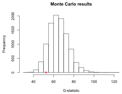
Fig. 1 Distribution of simulated G-statistics (* denotes actual value)
If a multinomial model exhibits a significant lack of fit, it means that one or more of the assumptions of the multinomial model have been violated. These are the same assumptions that are required for the binomial model.
The third violation can be partially addressed by including additional predictors to differentiate some of those observations or by including interactions of existing predictors. But beyond making the means model more complicated, dealing with lack of fit problems in a multinomial model is hard because software implementations of standard corrective measures are limited for multinomial models.
If we formulate the multinomial model as a Poisson model a number of additional options become possible. Violations of the multinomial assumptions translate into overdispersion in the Poisson model. Typical corrections of Poisson overdispersion include replacing the Poisson model with a negative binomial model, adding random effects, or fitting what's called a quasi-Poisson model. Because of the large number of auxiliary terms that are needed to make the conversion from multinomial model to Poisson, fitting a negative binomial model or a mixed effects model can be difficult. A quasi-Poisson model on the other hand is easy to fit. It just involves making a post hoc adjustment to the standard errors of the Poisson model by inflating them with a measure of the overdispersion, the Pearson deviance divided by its degrees of freedom.
In our current example, if we had found that the multinomial model did not fit, and assuming that adding more predictors and interactions did not help, we could refit the model as a quasi-Poisson model using the family=quasipoisson argument of glm.
To avoid looking at all of the coefficients in the summary table I use the grep function to locate those coefficients that contain "food" in their name. The first argument to grep is the pattern to search for and the second argument is the object to be searched. In the call below I search the row names of the coefficient matrix for the string 'food'.
The first four listed occurrences correspond to the main effects of food, so I skip those and extract the remaining entries from both the Poisson and quasi-Poisson models.
What we see is that the coefficient estimates of the two models are identical, but the reported standard errors of the quasi-Poisson model are larger to account for the overdispersion. This is a very crude correction but it is better than doing nothing. Of course for the current model we've already demonstrated that making this correction is unnecessary.
Because multinomial models generate a large number of parameter estimates, it is almost mandatory that we try to summarize the results using graphs. Panel graphs are ideally suited for this. There are a number of ways the results could be presented and in practice it might be useful to consider more than one.
As an illustration I summarize the lake effect on food choice using the results from the Poisson fit. As we discovered above these coefficients occupy rows 18:29 of the coefficient table. I extract that portion of the coefficient table as well as the corresponding portion of the variance-covariance matrix of the parameter estimates.
Currently the coefficients are organized in a way that facilitates comparisons across lakes for a given food preference. To compare food preferences within a lake we need to change this. We can sort the row names of the coefficient matrix or we can refit the model with the order of food and lake in the interaction term switched. I choose to sort the row names.
I collect the estimates and standard errors in a single data frame to which I add the two variables that make up the interaction term. An easy way of generating the variables is with the expand.grid function, It combines the different levels of two vectors in all possible ways.
The order created by expand.grid matches the row labels of the coefficient table.
I wish to display 95% confidence intervals for the log odds ratios as well as a second set of confidence intervals that permit making pairwise comparisons between the log odds ratios displayed in the same panel. I extract the functions and code for doing this from lecture 6.
I organize the remaining code as a function so that I can obtain confidence levels only for the estimates that will get displayed in a single panel. The four arguments of the function correspond to the row numbers of the out.mod data frame, the number of estimates being compared (4), the fitted glm model, and the variance-covariance matrix of the parameter estimates.
Because each panel displays four food type odds ratios there are six pairwise comparisons possible in each panel.
The confidence levels are quite variable. I begin by producing the graph using the smallest reported confidence levels for each panel. If a pairwise comparison does not show up as significant at this level then it will not be significant at any higher level either. On the other hand, pairwise comparisons that look to be significantly different at this setting could appear to be different only because the setting is too low relative to what it should be. Except for the changing the labels on the graph the code shown below is mostly unaltered from what was given in lecture 6.
I generate the lattice plot.
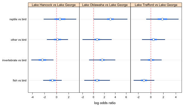
Fig. 2a Effect of lake on food choice log odds ratios (using smallest confidence levels)
In the output from the ci.func function, the smallest confidence levels correspond to the 1 vs 2 comparisons in panels 2 and 3, and the 1 versus 3 comparison in panel 1 (number 1 corresponds to the bottom of the panel). I examine things one panel at a time.
Panel 1
The 1 versus 3 comparison is not significant so we can raise the confidence level to the next lowest value, 0.5248087. This means recalculating the confidence intervals and then redoing the plot. The result is shown below (leaving out the lattice code).
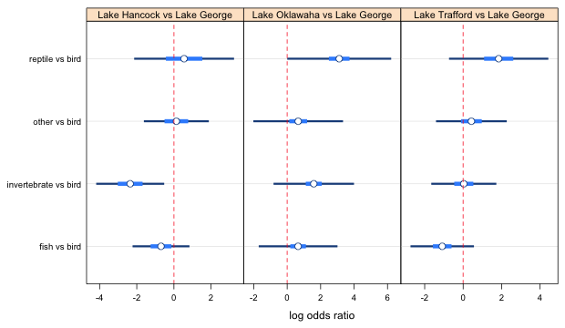
Fig. 2b Effect of lake on food choice log odds ratios (using 2nd smallest confidence level in panel 1)
At this point we see that the fish and invertebrate intervals do not overlap using the correct confidence level, so these two log odds ratios are clearly significant. The 1 versus 4 comparison is not significant. Raising the the confidence level to 0.7268 (the suggested value in the vals1 vector) will only increase the overlap, so we've completed the comparisons involving fish.
Turning to the remaining comparisons the "other" versus bird interval overlaps the reptile vs bird interval with the confidence level set at 0.52. If we raise it to the recommended level of 0.73 they will overlap even more. So, we don't have to do anything more with this one either. The only comparisons left to consider are invertebrate versus bird compared with other versus bird and reptile versus bird. Currently they don't overlap but we have the confidence levels set too low to be able to make these comparisons. I try changing the levels to their proper values and see if the intervals are still distinct.
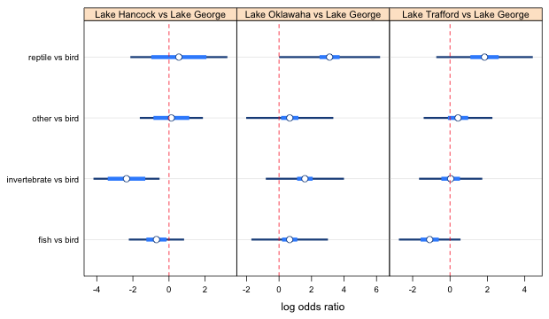
Fig. 2c Effect of lake on food choice log odds ratios (using the highest confidence level for panel 1)
From the graph, invertebrates versus bird is different from other versus bird as well as reptile versus bird. Changing this last level screwed up the fish and invertebrate comparison; they now overlap. A solution is to just use the previous settings with the confidence level set at 0.524, vals1[4] for all four points. The actual choice of confidence levels is not important as long as the correct relationships between the estimates are shown.
Panels 2 and 3
We still have to do the same thing separately for panels 2 and 3. I spare you the details and just list the results. In panel 2 it turns out that 1 is different from 4 but nobody else is significantly different. In panel 3, 1 turns out to be different from 2, 3, and 4, but no one else is different. The final settings I used to get all of these relationships to display correctly are given below and they are not unique. The specified levels don't follow much of a pattern except that they do seem to yield the correct display of the relationships between the different log odds ratios.

Fig. 3 Effect of lake on food choice log odds ratios (final choices for the confidence levels)
From Fig. 3 we see that two of the 95% confidence intervals for the log odds ratios don't include zero. Thus we can say that the odds of choosing invertebrates over birds is significantly lower in Lake Hancock than in Lake George. On the other hand the odds of choosing reptiles over birds is significantly higher in Lake Oklawaha than in Lake George. None of the remaining log odds ratios are statistically significant.
Using the pairwise confidence intervals we can look for differences among the food preference odds ratios for the same two lakes. We see that the odds ratio of choosing invertebrates over birds in Lake Hancock versus Lake George is significantly lower than the other three odds ratios for these two lakes: fish versus bird, "other" versus bird, and reptile versus bird. In the Lake Oklawaha versus Lake George comparison, the odds ratio for choosing fish over bird is significantly lower than the odds ratio of choosing reptile over bird. Finally in the Lake Trafford versus Lake George comparisons the odds ratio for choosing fish over bird is significantly lower than all three of the others: choosing invertebrate over bird, "other" over bird, and reptile over bird.
To plot odds ratios instead of log odds ratios we need to exponentiate the individual estimates and their confidence intervals everywhere they appear in the above code. This doesn't provide a useful picture for this example because some of the estimates are very imprecise. When we exponentiate them they end up dominating the display and making it difficult to draw comparisons across groups. To generate a picture that is at least semi-useful I truncated the confidence levels for the odds ratios at 30 and changed the plotting symbol for the point estimate. The changes are highlighted in the code below.
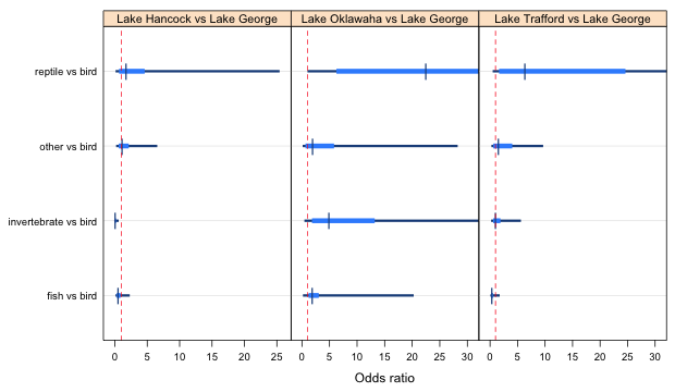
Fig. 4 Effect of lake on food choice odds ratios (truncated at the right)
The data set trees.csv is a portion of the North Carolina Vegetation Survey database and consists of the canopy cover values of individual woody plant species from various plots in North Carolina. Because of the difficulty of measuring canopy cover in the field, cover is often recorded on an ordinal scale. The categories used in this database and their roughly equivalent percentage values are: 1 = trace, 2 = 0–1%, 3 = 1–2%, 4 = 2–5%, 5=5–10%, 6 = 10–25%, 7 = 25-50%, 8 = 50–75%, 9 = 75–95%, 10=95–100%. A portion of the data set is shown below.
Because of inter-observer variability in measuring canopy cover there is interest in developing a regression model that can take as inputs the values of variables that are easily measured at ground level and generate an estimate of canopy cover. The variables U, V, and W in the trees data frame are examples of such variables.
For the purpose of this lecture we'll use W alone as a predictor of plot canopy cover.
As was discussed in lecture 39, one way to deal with ordinal data derived from an underlying continuous metric is to treat the scores as if they were measured on a ratio scale and then use them in an ordinary regression model. Based on the percentages these categories are supposed to represent it is pretty clear that the categories are not equally spaced (although they are approximately equally spaced on a log base 2 scale). Another approach is to assign to each category the midpoint of the underlying percentage range and again treat the result as if it were a continuous measure. We'll pursue a third strategy which is to treat these data as purely ordinal and carry out one of the variations of ordinal logistic regression discussed in lecture 39.
To simplify things I focus on a single species that is well-represented in the data set. There are 88 different plots in the data frame of which nine species occur in 70% or more of them.
Cornus florida was found in 85 of the plots and was recorded as having six different cover values. I use it to demonstrate fitting an ordinal logistic regression model.
A number of R packages can be used to fit the cumulative logit model. A straight-forward implementation is the polr function of the MASS package. The only new twist with this function is that it requires an ordered factor, created with ordered function, as the response variable.
Call:
polr(formula = ordered(truecover) ~ W, data = cornus)
Coefficients:
Value Std. Error t value
W 0.02684 0.005049 5.316
Intercepts:
Value Std. Error t value
2|3 -1.4356 0.3992 -3.5961
3|4 0.5211 0.3108 1.6764
4|5 2.1478 0.3962 5.4217
5|6 3.4230 0.5075 6.7444
6|7 4.9364 0.6753 7.3103
Residual Deviance: 247.6201
AIC: 259.6201
The polr function parameterizes the cumulative logit model as follows.
So, the polr function models the odds of having a cover value k or less versus having a cover value greater than k. Because of the negative sign in front of the regression coefficient a positive estimate for β means that increased values of W increase the odds of higher cover values. The reported value of β is 0.027 so we can say that large values of W favor the log odds of being in a larger cover class.
The cumulative logit model can also be fit with the VGAM package. This package is quite flexible in the variations of the cumulative logit model that it can fit. To match the sign of β from the polr function, we can use the following parameterization.
This parameterization is obtained with the vglm function by specifying cumulative in the family argument along with the settings of reverse and parallel as shown below.
Pearson Residuals:
Min 1Q Median 3Q Max
logit(P[Y>=2]) -2.2923 0.080029 0.168923 0.484102 0.65649
logit(P[Y>=3]) -4.5834 -0.908720 0.156884 0.645716 1.47533
logit(P[Y>=4]) -1.4444 -0.631251 -0.221531 0.369025 2.56225
logit(P[Y>=5]) -3.3772 -0.239888 -0.136126 -0.092288 4.10734
logit(P[Y>=6]) -1.7270 -0.169174 -0.088226 -0.060294 5.42472
Coefficients:
Value Std. Error t value
(Intercept):1 1.435673 0.4145891 3.4629
(Intercept):2 -0.520987 0.3087831 -1.6872
(Intercept):3 -2.147748 0.3826250 -5.6132
(Intercept):4 -3.422932 0.5032238 -6.8020
(Intercept):5 -4.936144 0.7169688 -6.8847
W 0.026834 0.0050751 5.2873
Number of linear predictors: 5
Names of linear predictors: logit(P[Y>=2]), logit(P[Y>=3]), logit(P[Y>=4]), logit(P[Y>=5]), logit(P[Y>=6])
Dispersion Parameter for cumulative family: 1
Residual Deviance: 247.6201 on 419 degrees of freedom
Log-likelihood: -123.8101 on 419 degrees of freedom
Number of Iterations: 6
The vglm function returns the same estimates as did the polr function except that while the sign of β is the same the signs of the individual intercepts are reversed.
The two models we've fit are both proportional odds models: they use a single coefficient to describe the effect of the predictor W. If we invert the logits and plot the probability curves of the five modeled probabilities we see the characteristic graphical signature of the proportional odds model. The curves are roughly parallel (except at their endpoints where they are constrained to be zero and one on a probability scale). The intercept shifts the curve to the left or right but the nature of the relationship with the predictor W is the same in each curve.
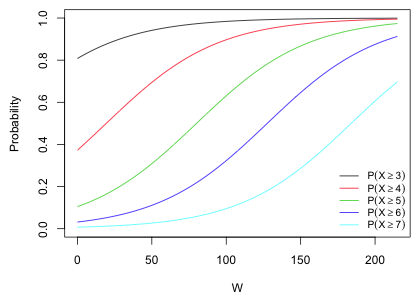
Fig. 5 Proportional odds assumption in the cumulative logit model
How might we use these results to address the original problem—finding a regression model to predict canopy cover? The probability expressions shown in Fig. 4 can be used to calculate the probabilities of the individual cover classes as follows.
The last expression follows because Cornus florida doesn't have a cover class greater than 7 in the data set. We can plot the estimated probabilities against W.
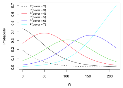
Fig. 6 Proportional odds assumption in the cumulative logit model
For each value of W we can pick the cover class with the highest probability or we can assign it a distribution of possible cover class values using the different probabilities shown. If we use the first option then, e.g., we would never assign cover class 2 to any observation.
The VGAM package provides a way to conduct an analytical test of the proportional odds assumption. We can fit the model that has separate slopes for each of the cumulative logit responses and compare it to the single slope model using a likelihood ratio test. The separate slopes model is obtained with the parallel=F argument. When we try to fit this model to the truecover response variable we receive a large number of warnings.
The warnings indicate that fitted values were obtained that were very close to zero. When we look at the summary output we see that the model apparently was estimated, but the log-likelihood is missing because a number of the estimated probabilities were so close to zero that their log was undefined.
Pearson Residuals:
Min 1Q Median 3Q Max
logit(P[Y>=2]) -2.8037 3.0091e-06 0.0019349 0.059714 1.4146
logit(P[Y>=3]) -23.3977 -7.0585e-01 0.1071105 0.405207 2.2853
logit(P[Y>=4]) -1.8237 -6.3842e-01 -0.1790875 0.262293 3.5736
logit(P[Y>=5]) -1.9461 -3.0320e-01 -0.1732860 -0.127485 3.0425
logit(P[Y>=6]) -1.2392 -2.0641e-01 -0.1447240 -0.114505 3.6850
Coefficients:
Value Std. Error t value
(Intercept):1 -0.4925839 0.7012324 -0.70245
(Intercept):2 -1.2911522 0.4262894 -3.02882
(Intercept):3 -2.3210544 0.4317115 -5.37640
(Intercept):4 -2.3009876 0.4302749 -5.34771
(Intercept):5 -2.9251780 0.6338667 -4.61482
W:1 0.2699540 0.1192624 2.26353
W:2 0.0592541 0.0138522 4.27760
W:3 0.0357884 0.0069295 5.16463
W:4 0.0149486 0.0051945 2.87776
W:5 0.0046051 0.0080005 0.57560
Number of linear predictors: 5
Names of linear predictors: logit(P[Y>=2]), logit(P[Y>=3]), logit(P[Y>=4]), logit(P[Y>=5]), logit(P[Y>=6])
Dispersion Parameter for cumulative family: 1
Residual Deviance: 220.7533 on 415 degrees of freedom
Log-likelihood: NA on 415 degrees of freedom
Number of Iterations: 10
The output indicates that the coefficient of W decreases dramatically as we move up cover classes. Curiously, even though there is no log-likelihood a deviance is reported. We can use the deviance to test the proportional odds assumption by comparing the deviance of this model with that of the proportional odds model.
The test is significant indicating a significant lack of fit. This result may be unreliable because of the warnings we obtained when fitting the model. Such warnings can arise if any of the categories have too few observations. That certainly could be the case here because the smallest and largest cover classes have only 8 and 5 observations respectively.
I try collapsing the two categories at the end with adjacent categories and refitting the two models.
The model with parallel=F still yields warnings about small fitted values. This time it did return a log-likelihood though.
The large difference in the log-likelihoods indicates that there is still a significant lack of fit. I carry out a formal test. (Note: the reported deviance is –2 times the reported log-likelihood.)
There is still a significant lack of fit. I try collapsing the categories even further.
The lack of fit is no longer significant. If we examine the coefficient tables we see that the separate slope estimates are fairly similar to the estimate of the common slope from the proportional odds model.
| Jack Weiss Phone: (919) 962-5930 E-Mail: jack_weiss@unc.edu Address: Curriculum for the Environment and Ecology, Box 3275, University of North Carolina, Chapel Hill, 27599 Copyright © 2012 Last Revised--April 29, 2012 URL: https://sakai.unc.edu/access/content/group/2842013b-58f5-4453-aa8d-3e01bacbfc3d/public/Ecol562_Spring2012/docs/lectures/lecture40.htm |