Lecture 6—Monday, January 23, 2012

Topics

• An error bar plot for pairwise comparisons
• Theoretical derivation
• Implementing the calculations in R
• Producing the error bar plot
• Cited references

R functions and commands demonstrated

• diag extracts the diagonal elements of a matrix.
• for defines a for loop, a programming tool that allows a set of instructions to be executed repeatedly, once for each value of a specified index vector. In R for loops are useful for short calculations but should never be used when the operations can otherwise be vectorized.
• numeric constructs a numeric vector.
• qt is the quantile function for a t-distribution.
• uniroot is used to find a root (zero) of a function over a specified interval.

An error bar plot for pairwise comparisons

You should recall from your elementary statistics course that a one-sample α-level significance test that tests whether the true value of a parameter is equal to zero is equivalent to determining whether the (1 – α)%-level confidence interval for that parameter contains zero. When we consider the two-sample case, testing the hypothesis that the two parameters are equal to each other, the two approaches are no longer equivalent. Using individual confidence intervals to carry out the two-sample hypothesis test leads to overly conservative results: one fails to reject the null hypothesis too often. The individual 95% confidence intervals can overlap even though a hypothesis test would conclude that the parameter values are significantly different at α = .05. This lack of equivalence is well-known and has been discussed repeatedly in the literature (Cumming 2009, Schenker and Gentleman 2001). The bottom line is that error bar displays of individual parameter estimates and their 95% confidence intervals cannot reliably be used to assess the statistical significance of differences between pairs of parameters.

A "solution" to this problem is to choose a confidence level for the individual confidence intervals that guarantees that non-overlapping pairs of confidence intervals do indicate statistically significant differences at α = .05. For independent parameters with roughly the same standard errors, the choice of 83.5% confidence intervals accomplishes this (Goldstein and Healy 1995, Payton et al. 2000, 2003). The more general case of dependent parameters has been discussed by Afshartous and Preston (2010) and their method can be adapted to our regression problem as I now demonstrate.

Theoretical derivation

The basic idea is simple. Under the null hypothesis of no significant difference between the parameters, we wish to choose a confidence level α for the individual confidence intervals such that the probability that they overlap is 0.95 (for a 5% test). Now,

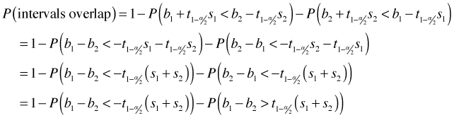
The two individual confidence intervals can fail to overlap in two distinct ways. Let b₁ and b₂ be two slopes from two different weeks that we wish to compare, let s₁ and s₂ be their respective standard errors, and let be the quantile of a t-distribution with degrees of freedom equal to the residual degrees of freedom of the regression model.

Fig. 1  b₁ < b₂ and the confidence intervals do not overlap

Fig. 1 shows the case when b₁ < b₂ and the confidence intervals fail to overlap. As the figure indicates the confidence intervals for the slopes from the two weeks don't overlap if the upper confidence limit of b₁ is strictly less than the lower confidence limit of b₂, i.e.,

.

The roles of b₁ and b₂ could be reverse with b₂ < b₁. In that case the confidence intervals don't overlap if the upper limit of b₂ is strictly less than the lower limit of b₁ so that

.

Thus we can write

I next carry out some algebra on these two inequalities starting by moving the parameters to the left side of the inequality.

In the last step I multiply both sides of the second inequality by minus one (thereby reversing the inequality).

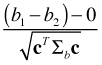
Recall from lecture 5 that b₁ – b₂ can be written as vector dot product.

In lecture 5 we also saw that the variance of this dot product is given by

where Σ_b is the variance-covariance matrix of b₁ and b₂. Under the null hypothesis that the mean difference of b₁ and b₂ is zero, the statistic,

,

the parameter estimate minus its mean divided by its standard error, is a z-statistic. When ordinary least squares is used to obtain the parameter estimates of a regression model, the difference b₁ –b₂ will have a normal distribution. Hence this z-statistic will have a t-distribution with degrees of freedom given by the residual degrees of freedom of the regression model. Using this fact the probability that the intervals overlap can be written as follows.

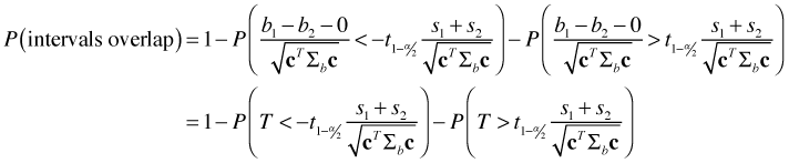
where T is a t-statistic. The only unknown in this expression is α which controls the confidence level of our individual confidence intervals. We need to choose α so that the probability that the intervals overlap is equal to 0.95.

Implementing the calculations in R

The R function below calculates the probability of interval overlap using the formula derived above. I write it as a function of three quantities: the unknown α-level, the regression model, and the variance-covariance matrix for the parameters being compared.

• The two t-statistic probabilities are calculated with the pt function. The expression pt(c,df) calculates P(T ≤ c). To obtain the reverse inequality I add the argument lower.tail=F, i.e., pt(c,df,lower.tail=F) = P(T > c). Note: for continuous random variables P(T ≤ c) = P(T < c).
• The t-quantile, , is calculated with the qt function: qt(1-alpha/2,df)
• To obtain s₁ + s₂ I use the diag function to extract the diagonal entries of the variance-covariance matrix sig, take their square root with sqrt, and sum the result: sum(sqrt(diag(sig))).
• The degrees of freedom needed for the various t-functions is contained in the df.residual component of the lm model object, model$df.residual.

I write a second function that takes this function evaluated at its arguments and subtracts 0.95 from it.

Finding the α that makes the nor.func1 function equal to 0.95 is the same as finding the α that makes the nor.func2 function equal to zero. The reason for reformulating things in this way is that there are standard protocols for finding the zeros of functions. In R there is a function called uniroot that will do this for us.

I next read in the data and fit the model. The model we need is the one I called mod3a. This is the re-parameterized version of model mod3 that returns the estimates and standard errors of the individual slopes and intercepts, rather than the differences from the reference group, week 1.

With four weeks of intercepts and slopes there are six pairwise comparisons we can make for each. I start by doing the calculations for the intercepts. I use the numeric function to initialize a vector with six slots, initially filled with zeros.

Next I extract the portion of the variance-covariance matrix that corresponds to just the four intercepts. This is the submatrix consisting of rows 1 through 4 and columns 1 through 4 of the matrix that is returned by vcov when applied to the lm model object.

To find the confidence levels needed for the six different pairwise comparisons I use a nested for loop. The outside loop chooses the first member of the comparison while the inside loop chooses the second member of the comparison. The index for the outer loop i runs from 1:3 while the index for the inner loop j runs from (i+1):4. The result is that each comparison is different and we do a total of six.

• ind is the index of the storage vector that I initialize to 1. At the end of the inner loop its value is incremented by one so that the next time through the loop the result of the calculation will be stored in the next location in the vector.
• sig is a 2 × 2 matrix containing the two variances and the covariance of the parameter estimates being compared.
• The uniroot function requires a function of one variable as its first argument and an interval in which to search for the root as its second argument. To make the nor.func2 function a function of one variable I make it a generic function using the function(x) notation where I make x the unknown α value we wish to find and I specify the regression model and variance-covariance matrix as the second and third arguments. The uniroot function returns a number of quantities but the number we want is contained in the $root component which I extract and store in the output vector.

The confidence levels are not all the same but they're fairly similar varying from 84.0% to 86.2%. So, each pairwise comparison requires a slightly different confidence level. This would be impossible to display graphically and when the values are this close will typically not make much of a difference, so I take the mean of the six values as the confidence level to use in constructing the individual confidence intervals. I round the value to three decimal places to avoid numerical problems with the confint function that will be used to calculate the confidence intervals.

I next repeat these calculations for the slopes. This involves choosing rows 5 through 8 and columns 5 through 8 of the variance-covariance matrix.

This time the confidence levels vary from 84.2% to 87.3% so once again the mean, 85.3%, is probably a reasonable choice for all six.

Producing the error bar plot

In lecture 5 we created a data frame out.mod that contained the variables we needed for the error bar plot.

I need to add to this the confidence intervals for the slopes and intercepts using the newly calculated confidence levels. Because the levels are slightly different for the slopes and intercepts I need to do two calculations and extract the intervals for the slopes from one and the intervals for the intercepts from the other.

I then add them as two new columns of the data frame out.mod first concatenating the intercept and slope left interval endpoints and then the right interval endpoints.

To produce the graph we can use the code from last time except that we need to add one more panel.segments call in the panel function to draw the error bars for the confidence intervals just calculated. Because they're shorter than the 95% confidence intervals I make them thicker and a lighter color.

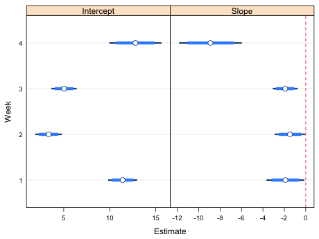
Fig. 2  Confidence intervals and point estimates of the slopes and intercepts from the regression model relating richness and NAP. Thin bars are 95% confidence intervals. Thick bars represent confidence intervals at confidence levels (here 85%) that permit making all pairwise comparisons between the different weeks.

Using the dark, skinny bars that are the 95% confidence intervals we see that all the slopes and intercepts are significantly different from zero. To make pairwise comparisons between the slopes and intercepts across different weeks we check to see whether the short, thick error bars overlap. In the slopes column we see that the slopes in weeks 1, 2, and 3 are not significantly different from each other but they are each significantly different from the slope in week 4. In the intercepts panel we see that the week 1 and 4 intercepts are not significantly different, and the week 2 and week 3 intercepts are not significantly different, but the week 1 and week 4 intercepts are both significantly different from each of the week 2 and week 3 intercepts.

Cited references

• Afshartous, D. and R. A. Preston. 2010. Confidence intervals for dependent data: Equating non-overlap with
  statistical significance. Computational Statistics and Data Analysis 54: 2296–2305.
• Cumming, G. 2009. Inference by eye: Reading the overlap of independent confidence intervals. Statistics in Medicine 28: 205–220.
• Schenker, N. and J. F. Gentleman. 2001. On judging the significance of differences by examining overlap between confidence intervals. The American Statistician. 55: 182–186.
• Goldstein, H. and Healy, M. 1995. The graphical presentation of a collection of means. Journal of the Royal Statistical Society, Series A 159: 175–177.
• Payton M. E., Miller, A. E. , and Raun, W. R. 2000. Testing statistical hypotheses using standard error bars and confidence intervals. Communications in Soil Science and Plant Analysis 31: 547–552.
• Payton, M. E., Greenstone, M. H., and Schenker N. 2003. Overlapping confidence intervals or standard error intervals: What do they mean in terms of statistical significance? 6pp. Journal of Insect Science 3: 34.

Course Home Page