Lecture 38—Monday, April 16, 2012

Outline of lecture

• Multinomial data
  • A connection between multinomial and Poisson distributions
• Types of multinomial models
• Baseline category logit model
  • Likelihood expression for the baseline category logit model
  • Alternatives to the baseline category logit model
• Fitting a multinomial model as a Poisson model

Multinomial data

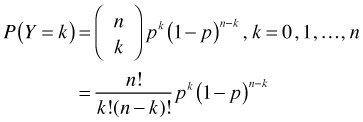
The multinomial distribution extends the binomial distribution to the case where there are more than two categories. If Y ~ binomial(n, p) then Y has the following probability mass function.

is called the binomial coefficient and is defined as shown. If we let Y₁ denote the number of successes and Y₂ the number of failures with probabilities p₁ and p₂, then an equivalent way to write the binomial probability mass function is the following.

where k₁ + k₂ = n and p₁ + p₂ = 1.

The multinomial model for a random variable Y with m categories is an obvious generalization of this last equation. Suppose is a multinomial random variable where Y₁, Y₂, …, Y_m are the frequencies of the m categories. The multinomial probability mass function with parameters n, p₁, p₂, … , p_m is the following.

where and . The term multiplying the probabilities is the called the multinomial coefficient and is defined as shown.

A connection between multinomial and Poisson distributions

There's a useful connection between the Poisson and multinomial distributions that allows one to fit regression models to multinomial data by assuming that the individual counts have separate Poisson distributions. This forms the basis for the classical statistical approach called the loglinear model.

Suppose Y₁, Y₂, …, Y_m are independent Poisson random variables with parameters λ₁, λ₂, …, λ_m. If we add the constraint that these m Poisson random variables must sum to a constant n, , then it follows that the conditional joint distribution of Y₁, Y₂, …, Y_m given n is multinomial.

It is easy to show that the sum of m independent Poisson random variables also has a Poisson distribution with parameter. Using this fact we can write the following.

where . Hence the conditional distribution is multinomial. The upstart is that multinomial regression models can be fit as Poisson regression models using maximum likelihood and we will obtain the same parameter estimates. As we'll see the Poisson approach requires estimating a lot of uninteresting auxiliary parameters that makes the this approach somewhat unwieldy. The advantage is that all the tools to account for observational heterogeneity that are available for Poisson models can be applied to the multinomial setting, even if such tools are not currently available for multinomial models per se.

Types of multinomial models

There are three standard multinomial models that are appropriate for different kinds of multinomial data.

1. Baseline category logit model. This approach is appropriate for nominal multinomial data in which the categories are purely labels. A nominal variable's values serve to identify membership in specific categories but have no other meaning.
2. Cumulative odds logit model. This approach can be appropriate for multinomial data in which the categories are ordinal. With ordinal categorical data the categories have a natural order. Examples include the following:
   1. Medical diagnoses such as "worse", "no change", "better"
   2. Likert scale categories such as "strongly disagree", "disagree", "neutral", "agree", "strongly agree"
   3. Braun-Blanquet and Daubenmire cover classes in botany

Ordinal data may derive from an underlying unobserved continuous scale (often viewed as representing a latent variable) that is difficult to record. Although ordinal categorical data are ordered a precise notion of distance is not well-defined. Thus we can say that one category is greater than another but not how much greater it is or even if the spacings of the different categories are the same.

3. Conditional logit model (also called a discrete choice model). These are often used in business or advertising but have seen some use in describing resource allocation in animals. The discrete choice model is defined not by the nature of the categories but by the kind of information we have about those categories and about the individual who chooses a category. The set of categories may change for each observation. What each observation has in common is a set of covariates that describe the different categories. There may be additional covariates that describe the chooser, the individual making the choice.

   In the discrete choice model we have predictors that describe the choices and additional descriptors that describe the chooser. In the baseline category and cumulative odds logit models we only have predictors that characterize the unit being categorized. A recent UNC graduate used a discrete choice model to describe the movement patterns of red cockaded woodpeckers from their nest tree. The categories were the possible flight paths a bird could take from its nest (which are different for birds at different nests). Each flight path was characterized by the amount of habitat of a specific type that it traversed. Additional information was available about the choosers: sex, age, size, etc. The goal was to determine what factors affected bird movement.

Baseline category logit model

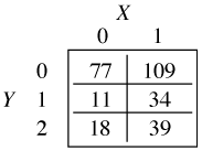
The baseline category logit model is also referred to as a multinomial logit model and polytomous logistic regression. As an illustration suppose a response variable Y has three categories 0, 1, and 2 and we have a single categorical predictor X with two categories 0 and 1. Our data can be organized in the form of a contingency table such as the one shown below.

If we only had two categories, say Y = 0 and Y = 1, we could construct the following odds directly from the above table.

• Odds of Y = 1 versus Y = 0 when X = 0:
• Odds of Y = 1 versus Y = 0 when X = 1:

Thus the odds ratio of category 1 versus category 2 for X = 1 versus X = 0 is the following.

Alternatively we could set this up as a logistic regression model.

from which the desired odds ratio is exp(β₁).

With three categories the situation is only slightly more complicated. We can choose one category as a reference category and construct log odds models that take the same form as in the two category case. With Y = 0 as the reference (baseline) group, we obtain the following log odds expression for Y = 1.

For Y = 2 we have the following.

Observe that each new log odds comparison generates a different set of regression coefficients, so response variables with many categories will generate a lot of parameters. With three categories, two log odds expressions are all we need because we can derive any other log odds comparisons from these two. For instance to compare Y = 2 against Y = 1 we proceed as follows.

The only complication in what we've done is that technically these aren't log odds. An odds is a ratio of the probability in favor of an outcome versus the probability against that outcome. In the above expressions the event in the denominator is not the complement of the event in the numerator. Thus these are better thought of as "odds-like" expressions. In some disciplines they're referred to as risk ratios. With these same caveats, if X is a dichotomous random variable coded 0 and 1 then exp(β₁₁) and exp(β₁₂) have "odds ratio" interpretations. In general if the denominator is chosen judiciously so that it represents a group that forms a natural reference group for comparisons then the baseline logit model will return probability ratios against an outcome of interest.

Likelihood expression for the baseline category logit model

For our simple example where Y = 0, 1, or 2, we can write down the conditional probabilities for Y = 1 and Y = 2 by exponentiating the two log odds expressions.

Because conditional probabilities must sum to 1 we obtain the following expression for .

Grouping the terms involving together and solving yields an expression for that only involves the regression parameters.

Plugging this into the formulas above we obtain expressions for the probabilities of Y = 1 and Y = 2.

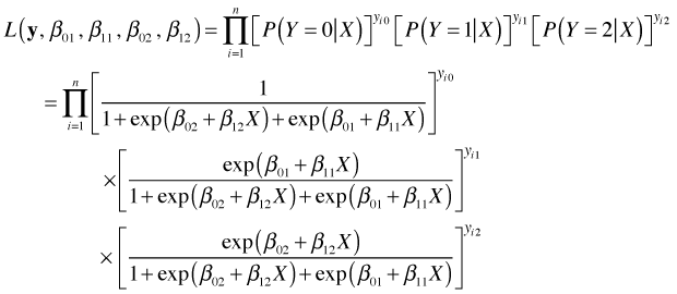
Let i = 1, 2, … , n denote the subjects. For subject i define the following dummy variables.

Using these we can write down the likelihood for the baseline logit model.

From this we can obtain maximum likelihood estimates of the baseline category logit parameters, likelihood ratio and Wald tests for individual parameters, and AIC for model comparison.

Alternatives to the baseline category logit model

An obvious alternative to fitting the baseline category logit model is to fit separate logistic regressions using only two categories at a time. Because the likelihoods for these two approaches differ so will the parameter estimates (although in the case of one dichotomous predictor the two approaches give the same estimates). In general the estimates one gets doing separate logistic regressions are less efficient (they tend to have larger standard errors). The usual recommendation is that if you choose to do separate logistic regressions then you should use as the reference category the one that has the largest prevalences.

Fitting a multinomial model as a Poisson model

Suppose we have multinomial counts organized in a data frame mydata as follows.

y x z freq
1 A a   n1
2 A a   n2
3 A a   n3
1 B a   n4
2 B a   n5
3 B a   n6
1 A b   n7
2 A b   n8
3 A b   n9

Here y is a multinomial response variable with three categories, x and z are two dichotomous predictors, and freq records the number of times that each combination of y, x, and z occurred. Baseline category logit models can be fit with the multinom function from the nnet package. To fit a baseline category logit model that is additive in x and z we would do the following.

multinom(y~x+z, weight=freq, data=mydata)

Any multinomial model with categorical predictors has a corresponding Poisson model that can be used to obtain equivalent tests of the effects of those predictors. Table 1 matches the R code of a multinomial model with the R code of its corresponding Poisson model (with the data argument left out). While the multinomial model uses the categorical variable as the response, the Poisson model uses the category counts as the response.

Notice that the Poisson model corresponding to the intercept-only multinomial model has four terms in it: the two predictors, x and z, as well as their interaction, x:z, plus the multinomial response, y. Predictors added directly to the multinomial model get added to the Poisson model as interactions with the response variable y. The likelihood and AIC of the Poisson and multinomial models are quite different but we can obtain the same statistical tests with each. If we wish to test the significance of the x effect in the multinomial model we can carry out the following likelihood ratio test.

anova(model1.mult, model2.mult, test='Chisq')

To test the effect of x using the Poisson models we need to test the significance of the y:x term in model 2.

anova(model1.pois, model2.pois, test='Chisq')

The differences in the deviances (log-likelihoods) in both the multinomial and Poisson frameworks are the same and yield the same test statistic.

One of the advantages of using the Poisson framework is that there are more tools for dealing with model violations. As we'll see one of the ways to assess lack of fit in a multinomial model is by comparing it to a saturated model. Lack of fit can arise from a violation of the one of the basic assumptions of the multinomial model (constant probabilities, independent trials) leading to what's called overdispersion. A quick fix for this in the Poisson framework is to include random effects or alternatively to fit a quasi-Poisson model instead of a Poisson. In the multinomial framework correcting for observational heterogeneity is much more difficult.

Course Home Page