Lecture 39—Wednesday, April 18, 2012

Outline of lecture

• Hypothesis testing in GAMs revisited
  • Method 1: Increase the number of knots
  • Method 2: Use the same smoothing parameters in both models
• Ordinal logistic regression
• A taxonomy of ordinal regression models
• The proportional odds assumption
• Discrete choice models
• Cited references

Hypothesis testing in GAMS revisited

In Final Exam, Part 2 I ask you to fit a GAM using all the predictors and then try to simplify it.

Formula:
Occupied_Unoccupied ~ s(TotalCanopy) + s(WildIndigoSize) + s(NearestWildIndigo) +
    s(DistanceNearestTree) + s(DirectionTree, k = 8) + s(Slope) +
    s(SlopeAspect, k = 8)

Parametric coefficients:
            Estimate Std. Error z value Pr(>|z|) 
(Intercept)  -0.6010     0.3566  -1.685   0.0919 .
---
Signif. codes:  0 ‘***’ 0.001 ‘**’ 0.01 ‘*’ 0.05 ‘.’ 0.1 ‘ ’ 1

Approximate significance of smooth terms:
                         edf Ref.df Chi.sq  p-value   
s(TotalCanopy)         3.409  4.249 31.697 2.96e-06 ***
s(WildIndigoSize)      1.000  1.000 32.884 9.79e-09 ***
s(NearestWildIndigo)   1.000  1.000  9.586  0.00196 **
s(DistanceNearestTree) 2.091  2.629  4.592  0.16224   
s(DirectionTree)       1.000  1.000  3.928  0.04749 * 
s(Slope)               1.000  1.000  0.054  0.81608   
s(SlopeAspect)         1.000  1.000  0.667  0.41416   
---
Signif. codes:  0 ‘***’ 0.001 ‘**’ 0.01 ‘*’ 0.05 ‘.’ 0.1 ‘ ’ 1

R-sq.(adj) =   0.58   Deviance explained = 53.1%
ML score = 116.83  Scale est. = 1         n = 328

The summary table suggests that Slope and SlopeAspect are not significant, but we know that the p-values of the Wald tests for GAMs can be quite unreliable. The different reduced models we might fit and compare against this one are not all equivalent because the variable SlopeAspect has a large number of missing values.

The gam function will silently remove these missing values anytime SlopeAspect is a predictor in the model. Models that are fit to different sets of observations cannot be compared using significance testing or AIC. Fortunately the anova function warns us if we try to compare models fit to different data.

It makes sense to test SlopeAspect first because if it can be dropped then the remaining variables can be examined using the full data set. To make models with and without SlopeAspect comparable I need to explicitly remove the observations that have missing values for SlopeAspect before fitting the model without SlopeAspect.

If we try to use the anova function to compare this model against the full model we get a surprise. Depending on the order the models are entered we either get a negative value for the change in deviance or a negative value for the difference in degrees of freedom and no reported p-value.

Model 1: Occupied_Unoccupied ~ s(TotalCanopy) + s(WildIndigoSize) + s(NearestWildIndigo) +
    s(DistanceNearestTree) + s(DirectionTree, k = 8) + s(Slope)
Model 2: Occupied_Unoccupied ~ s(TotalCanopy) + s(WildIndigoSize) + s(NearestWildIndigo) +
    s(DistanceNearestTree) + s(DirectionTree, k = 8) + s(Slope) +
    s(SlopeAspect, k = 8)
  Resid. Df Resid. Dev      Df Deviance Pr(>Chi)
1     317.2     211.64                         
2     316.5     212.64 0.70243  -1.0034        

Model 1: Occupied_Unoccupied ~ s(TotalCanopy) + s(WildIndigoSize) + s(NearestWildIndigo) +
    s(DistanceNearestTree) + s(DirectionTree, k = 8) + s(Slope) +
    s(SlopeAspect, k = 8)
Model 2: Occupied_Unoccupied ~ s(TotalCanopy) + s(WildIndigoSize) + s(NearestWildIndigo) +
    s(DistanceNearestTree) + s(DirectionTree, k = 8) + s(Slope)
  Resid. Df Resid. Dev       Df Deviance Pr(>Chi)
1     316.5     212.64                          
2     317.2     211.64 -0.70243   1.0034      

If we examine the log-likelihoods and AIC we see that we have apparently obtained the impossible. The more complicated of the two nested models has a lower log-likelihood.

The explanation for this is that the models we're comparing are not truly nested. Each model has its own set of smoothing parameters and these changed when the SlopeAspect variable was removed.

Apparently the presence of SlopeAspect put a constraint on the smoothing parameters of the other smooths that was lifted when SlopeAspect was excluded from the model. There are two ways to deal with this so that we can validly compare the models.

1. Increase the number of knots beyond the default value of 10 so that the smoothing parameters are not constrained by the presence or absence of SlopeAspect. Doing so will not make the models nested but it will make the models approximately nested.
2. Force the second model to use the smoothing parameters of the first model. With this choice the models will be truly nested and the likelihood ratio test will be valid.

Method 1: Increase the number of knots

To determine how many knots we should use, I fit both two models using a range of knot settings, record the log-likelihood and difference in deviances that are obtained, and determine at what point we start getting reasonable results.

With the choice of 20 knots the change in deviance is positive and the log-likelihood of the larger model exceeds the log-likelihood of the simpler model. Increasing the number of knots to 25 has only a small additional effect. I refit both models using k = 20 for all of the smooths where it is possible to do so. Slope is clearly linear so I leave it alone.

Model 1: Occupied_Unoccupied ~ s(TotalCanopy, k = k) + s(WildIndigoSize,
    k = k) + s(NearestWildIndigo, k = k) + s(DistanceNearestTree,
    k = k) + s(DirectionTree, k = 8) + s(Slope)
Model 2: Occupied_Unoccupied ~ s(TotalCanopy, k = k) + s(WildIndigoSize,
    k = k) + s(NearestWildIndigo, k = k) + s(DistanceNearestTree,
    k = k) + s(DirectionTree, k = 8) + s(Slope) + s(SlopeAspect,
    k = 8)
  Resid. Df Resid. Dev     Df Deviance Pr(>Chi)
1    317.46     213.44                        
2    316.42     212.53 1.0411   0.9129   0.3532

The results are now reasonable and we can conclude that SlopeAspect should be dropped.

Method 2: Use the same smoothing parameters in both models

We can make the models truly nested by forcing both models to use the same values of the smoothing parameters. The smoothing parameters are stored in the $sp component of the model object.

What's reported is the value of λ in the formula for smoothing splines.

Large values of λ correspond to smooths whose graphs are nearly a straight lines. We can force the reduced model to use the smoothing parameters of the full model by specifying them in the sp argument of the GAM. Because SlopeAspect has been removed from the simpler model, I need to specify only the first six smoothing parameters of the full model. The likelihood ratio test now returns a positive change in deviance and both the log-likelihoods and AICs have changed in the correct direction.

Model 1: Occupied_Unoccupied ~ s(TotalCanopy, k = k) + s(WildIndigoSize,
    k = k) + s(NearestWildIndigo, k = k) + s(DistanceNearestTree,
    k = k) + s(DirectionTree, k = 8) + s(Slope)
Model 2: Occupied_Unoccupied ~ s(TotalCanopy, k = k) + s(WildIndigoSize,
    k = k) + s(NearestWildIndigo, k = k) + s(DistanceNearestTree,
    k = k) + s(DirectionTree, k = 8) + s(Slope) + s(SlopeAspect,
    k = 8)
  Resid. Df Resid. Dev      Df Deviance Pr(>Chi)
1    317.49     213.44                         
2    316.50     212.64 0.99023  0.79671   0.3686

In practice it is probably a good idea to use both of these approaches in combination. The number of knots should be set large enough so that the smooths are not being constrained and a common value of the smooths should be chosen to ensure that the models being compared are truly nested.

Ordinal logistic regression

Ordinal logistic regression is a regression model for ordinal multinomial data that tries to take into account the natural order of the categories. Ordinal data can be analyzed using the baseline category logit model but at the expense of losing information contained in the order of the categories. Historically ordinal data have been treated as weakly numeric data. Scores were assigned to individual categories and a mean score calculated for each multinomial observation. The mean scores were then modeled as a function of predictors.

As an example Likert scales used in course evaluations often have numeric values associated with the categories (Table 1).

Associating numeric scores with category labels encourages raters to assign ratings that are commensurate with the numeric values. Numeric scores for use in a regression analysis can also be developed post hoc. There are two problems with treating ordinal data as if they were continuous.

1. Results can differ if a different scoring system is used. This places a burden on the analyst to demonstrate that the obtained results are score independent.
2. A scoring system imposes a distance metric on the categories that may not correspond to the metric that was used by the raters.

Modern approaches account for the order of ordinal data but don't impose a distance metric on the categories. They all tend to be modifications of the baseline category logit model in which two adjustments that are made to take advantage of the ordinal nature of the data.

1. Odds are reformulated so that they are true odds, not "odds-like" quantities. These odds are created to capture the directionality of the categories.
2. Ordinal data make it possible to describe the effects of predictors more parsimoniously by using the same regression coefficients in different odds comparison. This is called the uniform association, proportional odds, or parallel assumption.

Different odds formulations for ordinal data can be used with or without the assumption of parallelism, so these two adjustments are more or less independent of each other. Ordinal regression models are classified by the kind of odds they model. The choice depends on selecting which event comparisons are considered interesting. Once this choice is made, true odds are calculated as the ratio of the probability in favor of the event to the probability against the event.

A taxonomy of ordinal regression models

Although a number of R packages exist that can fit one or more types of ordinal regression models, the most comprehensive among these is the VGAM package (Yee 2010). With VGAM all of the standard ordinal regression models can be fit using a common syntax. Table 2 lists the basic ordinal regression models, the probabilities and odds they choose to model, and the corresponding VGAM syntax needed to fit these models.

Model	Probability	Odds	VGAM family
Cumulative odds			cumulative(reverse=T)
			cumulative
Continuation ratio			cratio
			sratio
Adjacent category			acat

1. In the cumulative odds models we collapse the multinomial categories into two categories in such a way that the order of the original categories is preserved. There are two ways to formulate the odds, as the probability of reaching and exceeding a given category divided by the probability of not achieving that category or what is essentially its reciprocal. For J categories there are J – 1 such comparisons one can make. For instance, if Y = 1, 2, 3, or 4 then we could make the following three comparisons: Y ≤ 1 versus Y > 1, Y ≤ 2 versus Y > 2, and Y ≤ 3 versus Y > 3.
2. The continuation ratio formulation yields a quantity that is analogous to the hazard function from survival analysis. In the version shown in Table 2 we restrict the set of interest to be those categories that equal or exceed the category of interest. So the reference group corresponds to those who do as well better than you. If we think of the categories as indicating progress then the continuation ratio per se (VGAM cratio) yields the odds of progressing (moving on) versus staying where you are. The VGAM sratio (stopping ratio) yields the odds of not progressing given that we've made it this far. The continuation ratio formulation is popular in educational research where, e.g., learning level is the ordinal categorical variable and the goal is estimate the probability of progressing beyond one's current level.
3. The adjacent category formulation focuses on the transition between adjacent categories. The regression model attempts to find predictors that affect this transition.

The proportional odds assumption

When we fit any of the ordinal models described in Table 2 to a response variable with J categories, we get J – 1 regression coefficients for each predictor. This is as many regression coefficients as we would get had we instead fit the baseline category logit model. The log odds for category j in a cumulative odds regression model with two predictors would be written as follows.

This yields J – 1 different intercepts, J – 1 different coefficients for x, and J – 1 different coefficients of z, one for each of the J – 1 odds comparisons we're making.

The usual choice in ordinal logistic regression is to retain the J – 1 different intercepts, but to have just single coefficients, β₁ and β₂, for the predictors x and z. This is called the uniform association, proportional odds, or parallel hypothesis because it assumes the logit curves for the different category transitions are parallel.

The proportional odds model is directly analogous to the ordinary regression model. With it we can speak of "the" effect of x and "the" effect of z on the response variable rather than having a different effect at each category transition. When someone reports that they carried out ordinal logistic regression they almost always mean they fit a cumulative odds logit model in which the assumption of parallelism was made.

It is important to recognize that the uniform association hypothesis is an assumption that needs to be examined. Generally the more predictors there are in an ordinal logistic regression model, the more likely it is that the assumption is being violated by at least one of the predictors. In very simple regression models with a single dichotomous predictor an easy way to check the uniform association hypothesis is to calculate the raw empirical odds ratios to see if they are approximately the same for different category transitions.

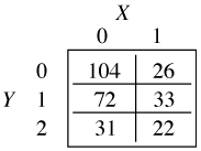
As an illustration consider the following toy example of an ordinal response variable Y with three categories and a dichotomous predictor X. The tabulated data are shown below.

Suppose we consider probabilities of the form , j = 0, 1, with the goal of fitting a cumulative odds logit model with the parallelism assumption. Without the parallelism hypothesis our model is the following.

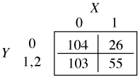
which yields two different odds ratios for X, exp(β₁₁) for the transition from Y = 0 to Y = 1 and exp(β₁₂) for the transition from Y = 1 to Y = 2. When j = 0 in the cumulative logit model we calculate the odds of Y ≤ 0 versus Y > 0. To obtain this the categories 1 and 2 of the contingency table are combined.

The odds ratio X = 1 versus X = 0 is calculated as follows.

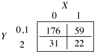
When j = 1, we calculate the odds of Y ≤ 1 versus Y > 1. This time categories 1 and 2 of the contingency table are collapsed.

The odds ratio for X = 1 versus X = 0 is calculated as follows.

We see that the two raw odds ratios are approximately the same suggesting that exp(β₁₁) ≈ exp(β₁₂) and hence that the separate coefficients β₁₂ and β₁₂ can be replaced by a single value β₁. This provides empirical evidence for the parallelism hypothesis for these data.

In the VGAM package we can test the parallelism hypothesis directly by comparing two ordinal regression models.

1. An ordinal regression model in which a common regression parameter for a predictor x is used for all categories of Y (parallel = T).
2. An ordinal regression model in which separate regression parameters for a predictor x are used for the different categories of Y (parallel = F).

These two models can be compared with a likelihood ratio test and if the test statistic is significant the parallel hypothesis is rejected. The general consensus is that this test may be overly conservative, rejecting the parallelism assumption too often. Given that a polytomous logit model will often fit the data better, it's probably prudent to examine the separate coefficients to see if the differences between them are substantive enough to reject parallelism.

In the end parallelism may be rejected for some predictors in a regression model but not all. In such a case it is possible to fit a model in which some predictors have a single coefficient for all categories of the response while other predictors have different coefficients. Such a model is called a partial proportional odds model and it too can be fit with the VGAM package.

Discrete choice models

In the typical discrete choice model we have a number of subjects making choices along with predictors that characterize the subjects as well as predictors that characterize the choices. The choice sets may vary across subjects so that we don't have a fixed set of multinomial categories. A place where discrete choice models have been used in ecology is in animal resource allocation studies. Although different animals will have different resources from which to choose, they are linked by a common set of predictors that characterize the resources and a common set of predictors that characterize the choosers. The notation for discrete choice models is given in Table 3.

Term	Definition
Ci	the set of choices available to subject i
	the vector of values of the p explanatory variables describing subject i and choice j
	the probability that subject i chooses choice j

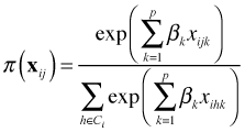
The discrete choice model uses the following expression for .

This expression has its origin in utility theory in economics. Notice that it has the same form as the Cox partial likelihood from survival analysis. Instead of summing over the risk set in the denominator we sum over the choice set. Because of the close similarities between the discrete choice model and the Cox model, we can use survival analysis software to specify the discrete choice likelihood and obtain parameter estimates. It's important to realize that this is just a device for obtaining parameter estimates. There is no survival function interpretation for the results.

For example, suppose we have two subjects making choices. Subject 1 has a choice set {A, B, C} and subject 2 has a choice set {B, C, D}. Predictors x1 and x2 provide information about the choices and/or subjects. Suppose subject 1 chooses A and subject 2 chooses C. To determine how predictors x1 and x2 influence these choices we fit a discrete choice model in which we organize the data as shown in Table 4.

The variable Choose indicates the option that was selected by the subject, Choose = 1, and the options that were rejected, Choose = 0. This variable plays the role of the censor variable in survival analysis. The option that is chosen is assigned Time = 1, while all the options not selected are assigned Time = 2. This forces all of the remaining choices to be in the risk set at the "time" the choice was made. To ensure that the probabilities and risk sets are calculated separately by subject, we make each subject a stratum here denoted by the variable Bout. This discrete choice model can be fit with the coxph function of the survival package as follows.

coxph(Surv(Time, Choose) ~ x1 + x2 + strata(Bout))

A paper that introduces discrete choice modeling to ecologists is Cooper and Millspaugh (1999).

Cited references

• Cooper, A. B. and J. J. Millspaugh. 1999. The application of discrete choice models to wildlife resource selection studies. Ecology 80: 566–575.
• Yee, T. W. 2010. The VGAM package for categorical data analysis. Journal of Statistical Software 32(10): 1–34. URL http://www.jstatsoft.org/v32/i10/.

Course Home Page