Assignment 4—Solution

Question 1

Method 1

Following the hint I use the strsplit function to split the elements of the trt variable into individual components. For the split argument I enter two quotes with nothing between them.

[[2]]
[1] "O"

[[3]]
[1] "O"

[[4]]
[1] "P"

[[5]]
[1] "P"

[[6]]
[1] "P"

[[7]]
[1] "P" "K"

[[8]]
[1] "P" "K"

The object that strsplit creates is called a list. Lists are a generalization of data frames in which the individual components can have different lengths as well as be different kinds of objects. To access an individual element of a list we need to use the double bracket notation.

If we use the intersection operator, %in%, to determine if the character 'L' is in the list we get an uninformative answer.

It just tells us that 'L' was found somewhere in the list, not where it was found. To determine the locations of 'L' we need to operate on each element of the list separately. The sapply function will do that for us. If we make the list, out.sp, the first argument of sapply then the function we specify in the second argument will be applied to each element of out.sp separately. The function we need is the following: function(x) 'L' %in% x. Each time a different element of the list is inserted as the variable x.

A second way of obtaining the same result is to make the 1:48 the first argument of sapply (where 48 is the number of elements in the list). Then the function becomes: function(x) 'L' %in% out.sp[[x]]. This time the numbers 1 through 48 will be inserted sequentially for x and the corresponding element of the list will be tested to see if 'L' is an element.

With this output we can use the ifelse function to conditionally assign the values 'present' or 'absent' to a new variable as follows.

We repeat this for the three remaining factors assigning the results to a variable.

Method 2

R has a number of search and replace functions. One of these is grep. The grep function takes a string to search for as its first argument and the object to search as the second argument. If the second argument is a vector grep gives us the index numbers of the entries in the vector where the string was found.

We can use this as follows. First we create a new character variable all of whose values are 'absent'.

Next we change the entries whose indices were returned by grep to 'present'.

Finally we convert the result to a factor.

To create the other factor variables we repeat these three steps for 'N', 'P', and 'K'.

Question 2

Checking for block × treatment interaction

The design is a randomized block design with no replication of treatment within block. Although we can't formally test for a block × treatment interaction we can examine the patterns graphically. I use the interaction.plot function to plot the treatment means separately by block to see if there are any obvious patterns.

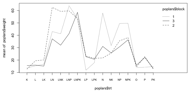
Fig. 1  Interaction plot of the block × treatment effects

With 16 treatments perfect parallelism of the profiles is difficult to achieve. Fig. 1 shows some crisscrossing of the profiles indicating the effects are not the same across blocks. There are clearly some issues here but with only three blocks it's difficult to determine how serious to take this. Some of the crisscrossing is just random noise and/or involve treatments or effects that are not significant. The one positive thing one can assert is that the basic pattern of treatment effects (which ones have large effects and which ones have small effects on the response) appears to be more or less consistent in the three blocks.

With only three blocks we don't have much power to carry out a formal test for specific kinds of interaction. We can carry out the Tukey test for non-additivity as follows.

Response: weight
              Df  Sum Sq Mean Sq F value   Pr(>F)   
factor(block)  2   215.4  107.72  1.5932   0.2205   
trt           15 10310.1  687.34 10.1658 8.07e-08 ***
ab             1    61.9   61.89  0.9154   0.3466   
Residuals     29  1960.8   67.61                     
---
Signif. codes:  0 ‘***’ 0.001 ‘**’ 0.01 ‘*’ 0.05 ‘.’ 0.1 ‘ ’ 1

So, the product term is not significant. We can reject the presence of a multiplicative interaction between block and treatment effects.

Fitting the randomized block design model

I start by fitting the fixed effects version of the randomized block design including the four-factor interaction of the factors L, N, P, and K.

Response: weight
              Df Sum Sq Mean Sq  F value   Pr(>F)   
factor(block)  2  215.4   107.7   1.5978 0.219094   
L              1  884.9   884.9  13.1254 0.001064 **
P              1  354.8   354.8   5.2623 0.028968 * 
N              1 8350.3  8350.3 123.8513 3.58e-12 ***
K              1   43.9    43.9   0.6510 0.426106   
L:P            1    2.0     2.0   0.0303 0.863014   
L:N            1  395.0   395.0   5.8590 0.021761 * 
P:N            1  108.3   108.3   1.6063 0.214763   
L:K            1   23.4    23.4   0.3468 0.560354   
P:K            1   20.7    20.7   0.3066 0.583876   
N:K            1    2.8     2.8   0.0409 0.841163   
L:P:N          1    1.3     1.3   0.0193 0.890482   
L:P:K          1    1.4     1.4   0.0213 0.884976   
L:N:K          1    4.1     4.1   0.0614 0.805936   
P:N:K          1   79.8    79.8   1.1840 0.285216   
L:P:N:K        1   37.3    37.3   0.5529 0.462924   
Residuals     30 2022.7    67.4                     
---
Signif. codes:  0 ‘***’ 0.001 ‘**’ 0.01 ‘*’ 0.05 ‘.’ 0.1 ‘ ’ 1

For comparison I fit a model using the nlme package in which blocks are treated as random.

The results are identical. Based on the ANOVA table we can drop the four-factor and all the three-factor interactions. It appears that the only significant two-factor interaction is the L:N interaction. (Note: The reported test of blocks in the lm output is not appropriate. The error term in the model is the block × treatment interaction and isn't an appropriate measure of background variability for testing the block effect. In any case, we should retain the block term in the model because it is part of the experimental design.)

Because the data are balanced the order we fit the terms doesn't matter, so I drop all the non-significant 2-factor interactions too.

The main effect of K is not significant so I drop it leaving the following model.

Question 3

I examine the summary table of the final model.

Random effects:
 Formula: ~1 | block
        (Intercept) Residual
StdDev:    1.775939 7.567076

Fixed effects: weight ~ L * N + P
                     Value Std.Error DF  t-value p-value
(Intercept)       12.75625  2.648767 41 4.815919  0.0000
Lpresent           2.85000  3.089246 41 0.922555  0.3616
Npresent          20.64167  3.089246 41 6.681782  0.0000
Ppresent           5.43750  2.184427 41 2.489212  0.0170
Lpresent:Npresent 11.47500  4.368853 41 2.626547  0.0121

In the final model there is a significant main effect due to P and a significant interaction between L and N. The effect of each nutrient is to increase new growth. P increases growth by 5.4 g. L alone increases growth by 2.8 g, N alone increases growth by 20.6 g. The combination of L and N together increase growth by an additional 11.5 g over what each of these soil additives contributes alone.

Question 4

Because there is a significant two-factor interaction between L and N, the graph we construct should focus on explicating the nature of that interaction. Because there is only a main effect of P, the effect of P will only be to shift the two-factor interaction vertically. Thus it makes sense to display the results of the experiment as a panel graph in which each panel shows a different level of P while the panel itself displays the interaction between L and N.

I begin by constructing a data frame that contains the four different ways of combining the levels of L and N.

I next write a function to generate the regressors of the regression model.

I next write a second function that applies the cvec function to the matrix g that contains the various ways of combining the levels of L and N for a specific value of P to produce a matrix of the values of the model regressors. I generate two matrices: one for the case when P is absent and the other for when P is present.

To calculate difference-adjusted confidence intervals we need the function from lecture 8.

Technically this function is only appropriate for large samples. For small samples the normal approximation is suspect and we should probably use a t-distribution. Recall though that there is an issue with how to correctly calculate degrees of freedom in mixed effects models. The lme function does return the degrees of freedom it uses for its tests. They're contained in the $fixDF$X component of the model.

If we compare the normal quantile to the quantile of a t-distribution with 41 degrees of freedom we see that there is a noticeable difference.

To use these we'd have to replace the qnorm and pnorm functions in ci.func2 with qt and pt and add an argument that specifies the degrees of freedom. The effect that using the normal distribution rather than the t-distribution will have on the confidence intervals is that our intervals based on the normal distribution will be about 0.15 units too short.

I obtain the variance-covariance matrices of the means separately for the two different values of P.

I run the ci.func2 function and find that a 75% confidence interval should be used for the difference-adjusted confidence levels.

I modify the make.data function from lecture 8 to generate a data frame of means, standard errors, and confidence intervals. The changes are highlighted.

I generate the results separately for the two values of P and combine the results into a single data frame.

The only change we need to make to the groups panel function is in the panel function that produces the grid lines.

The prepanel function needs no changes.

The changes I made to the xyplot call are highlighted.

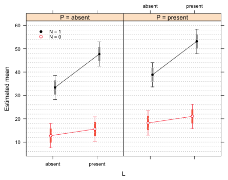
Fig. 2  Interaction plot with 75% difference-adjusted confidence intervals

To verify that the graph is correct we can compare the inferences we would draw from the graph to what is shown to the summary table of the model.

Random effects:
 Formula: ~1 | block
        (Intercept) Residual
StdDev:    1.775939 7.567076

Fixed effects: weight ~ L * N + P
                     Value Std.Error DF  t-value p-value
(Intercept)       12.75625  2.648767 41 4.815919  0.0000
Lpresent           2.85000  3.089246 41 0.922555  0.3616
Npresent          20.64167  3.089246 41 6.681782  0.0000
Ppresent           5.43750  2.184427 41 2.489212  0.0170
Lpresent:Npresent 11.47500  4.368853 41 2.626547  0.0121

1. The L effect (when N = 0) is not significant (p = 0.36). This correctly corresponds to the overlapping 75% confidence intervals of the N = 0 profile.
2. The N effect (when L = 0) is significant (p < .0001) and this corresponds to the non-overlapping 75% confidence intervals of the two N profiles when L = 0.
3. The L:N interaction is significant (p = 0.01). This is not directly visible from the graph but if we were to translate the N = 0 profile so that it overlaps the N = 1 profiles, the two 75% confidence intervals for L = 1 would fail to overlap.
4. The P effect is significant (p = 0.01). When we examine the graph we see that the corresponding 75% difference-adjusted interval pairs in the two P panels overlap. Thus the choice of a 75% interval does not allow us to draw correct conclusions when we compare observations across panels.

If we wish to present a panel graph in which the reader is allowed to make all pairwise comparisons then we'll need to find the appropriate confidence levels using all eight means. I recreate the g matrix of unique predictor combinations, the corresponding matrix of regressor values cmat, and calculate the difference-adjusted confidence levels.

Three different confidence levels are shown. The 0.75 level should be used to compare means in the same panel. The 0.58 level should be used to compare means in different panels (different values of P) that have the same values of L and N. The 0.84 level should be used to compare means in different panels (different values of P) in which one or both of the levels of L and N are different.

Because the graph we're constructing is just a tool for summarizing the model it may not be necessary to use all three confidence levels. I redo the interaction plot using 84% confidence levels to see if they're needed or whether the 75% intervals would suffice. I redo the the make.data function for this purpose.

Fig. 3  Interaction plot with 84% difference-adjusted confidence intervals

If we make the cross-panel comparisons permitted by these intervals we see that all the pairwise comparisons are significant. This is the same conclusion we would have drawn by using the shorter 75% intervals, therefore we don't need to show both. The 75% intervals are sufficient for drawing the correct inferences.

Finally I examine the 58% intervals. This time I add them to Fig. 2 so that the 95% , 75%, and 58% intervals are all shown. I redo the make.data function so that all three intervals are created. I also modify the group panels function to add these new intervals for each group.

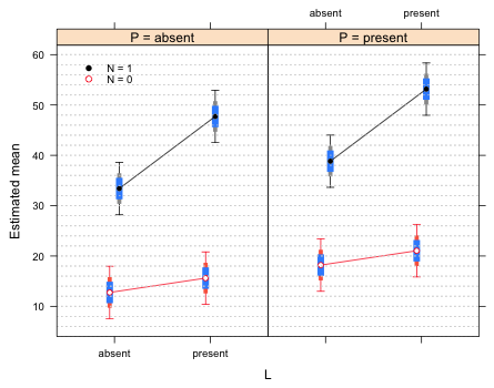
Fig. 4  Interaction plot with 58% and 75% difference-adjusted confidence intervals

The 58% intervals of means with the same values of L and N but different values of P do not overlap, which is correct. If we were to use the 58% intervals, rather than the 75% intervals, to make comparisons within the same panel we see that we would draw the same conclusions as we do with the 75% intervals. Therefore we don't need both of them. I redraw the graph using only 58% difference-adjusted confidence intervals.

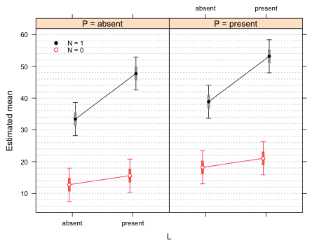
Fig. 5  Interaction plot with 58% difference-adjusted confidence intervals

Course Home Page