So far we've studied regression models for two data types:
For continuous data we assumed that a reasonable data generating mechanism for the observed values was a normal distribution and we used an ordinary regression model to determine how the mean of that normal distribution varied as a function of the values of various predictor variables. For count data standard data generating mechanisms are the Poisson distribution and the negative binomial distribution. To ensure that our regression model returned non-negative estimates for the mean of these distributions we constructed a regression model for the log of the mean. We refer to the log function in this context as the link function for count data.
We now turn to regression models for binary data. Binary data are data in which there are only two possible outcomes: 0 and 1, failure and success. Thus we are dealing with purely nominal data. The simplest case of binary data is when we have a single observed binary outcome. A textbook example of this is flipping a coin once and recording the outcome, heads or tails.
The standard probability model for such a simple experiment is the Bernoulli distribution. The Bernoulli distribution has one parameter p, the probability of success, with 0 ≤ p ≤ 1. The notation we will use is ![]() , to be read "X is distributed Bernoulli with parameter p." Obviously if the probability of success is p, then the probability of failure is 1 – p. The mean of the Bernoulli distribution is p. The variance of the Bernoulli distribution is p(1 – p). We refer to the single binary outcome as a Bernoulli trial.
, to be read "X is distributed Bernoulli with parameter p." Obviously if the probability of success is p, then the probability of failure is 1 – p. The mean of the Bernoulli distribution is p. The variance of the Bernoulli distribution is p(1 – p). We refer to the single binary outcome as a Bernoulli trial.
Binary data don't become interesting statistically until an experiment produces multiple Bernoulli trials. Depending on how we choose to record the results from this experiment we are led to one of two closely related probability models: the product Bernoulli distribution or the binomial distribution.
The product Bernoulli distribution is the natural model to use when we observe a sequence of n independent Bernoulli trials each with some probability of success pi. An example of this in ecology would be the construction of a habitat suitability model for the spatial distribution of an endangered species. Typically we record the presence or absence of the species in a habitat in each of a set of randomly located quadrats. We then try to relate the observed species distribution to measured characteristics of the habitat. Each individual species occurrence is treated as the realization of a Bernoulli random variable whose parameter p is modeled as a function of habitat characteristics.
Suppose ![]() are n independent binary outcomes from such a habitat suitability study. Let the observed binary outcomes be x1 = 1, x2 = 0, x3 = 0, x4 = 1, … , xn = 1 for quadrats numbered 1, 2, 3, … , n. To formulate the likelihood of our data we begin by writing down the probability of observing the data we obtained, the joint probability of our data.
are n independent binary outcomes from such a habitat suitability study. Let the observed binary outcomes be x1 = 1, x2 = 0, x3 = 0, x4 = 1, … , xn = 1 for quadrats numbered 1, 2, 3, … , n. To formulate the likelihood of our data we begin by writing down the probability of observing the data we obtained, the joint probability of our data.
where in the second step we make use of the fact that the individual binary outcomes are assumed to be independent. If we've measured a common set of predictors that vary among the binary observations we can develop a regression model for p as a function of these predictors. We then replace the various pi in the log-likelihood by their corresponding regression models and obtain maximum likelihood estimates of the regression coefficients.
Another common way binary data arise involves a slight variation of the product Bernoulli scenario. Suppose instead of observing the individual outcomes from the independent trials we only observe the number of successes. The classical example of this is an experiment in which a coin is flipped n times and we record the number of heads, but not the order in which the heads and tails appeared. Because we've haven't recorded the information about the individual binary trials we are forced to assume (unlike the product Bernoulli model) that the probability of a success p is the same for each of the n trials.
A simple biological illustration of this might be a seed germination experiment. Suppose in such an experiment 100 seeds are planted in a pot and the number of seeds that germinate is recorded. Suppose we observe that k out of 100 seeds germinated. In this case we haven't recorded which seeds germinated only that k of them did. If we had recorded the order of the events (i.e., which seed yielded which success or failure) then the product binomial model would be appropriate. Now there are many different ways that k successful germinations could have occurred. The first k seeds could have been successes while the last 100 – k were failures, or the first 100 – k seeds could have been successes and the last k were failures, and there are many others. Each of these possible events is contributing to the overall probability of obtaining the k observed successes. Because the seeds are assumed identical each such outcome has the same probability that is given by the product Bernoulli model:
![]()
where I replace pi by p because the probabilities are the same on each Bernoulli trial. So all we need to do is figure out how many of these different outcomes each leading to k successes there are and multiply that number by their identical probability. The answer is provided by the binomial coefficient whose derivation is given in any elementary probability text.
Putting this altogether the probability of observing k successes out of n independent trials where the probability of success p is the same on each trial is given by the binomial probability mass function.
Formally a binomial random variable arises from a binomial experiment, which is an experiment consisting of a sequence of n independent Bernoulli trials. If ![]() are independent and identically distributed Bernoulli random variables each with parameter p, then
are independent and identically distributed Bernoulli random variables each with parameter p, then
![]()
is said to have a binomial distribution with parameters n and p. We write this as ![]() . Given the mean and variance of the Bernoulli distribution it should not be surprising that the mean of the binomial distribution is np and the variance of the binomial distribution is np(1 – p). To better distinguish the binomial distribution from the product Bernoulli distribution, we sometimes refer to data arising from a binomial distribution as grouped binary data.
. Given the mean and variance of the Bernoulli distribution it should not be surprising that the mean of the binomial distribution is np and the variance of the binomial distribution is np(1 – p). To better distinguish the binomial distribution from the product Bernoulli distribution, we sometimes refer to data arising from a binomial distribution as grouped binary data.
In order for an experiment to be considered a binomial experiment four basic assumptions must hold.
If (1) or (2) are violated then a binomial model is completely inappropriate and a different probability distribution should be used. If (3) is violated, it may be possible to salvage things by including random effects in the final model. If (4) is violated it may be possible to account for it by adding a correlation structure to the model.
The dbinom function of R is the probability mass function for the binomial and it returns the probability of a specified value. The syntax of dbinom is dbinom(x, size, prob) where size is what we have been calling n and prob is what we've been calling p. I start by placing three binomial distributions side-by-side. All have n = 10, but p varies with p = 0.1, 0.5, and 0.9. I use the mfrow argument of the par function of R to obtain a graphical display consisting of 1 row and 3 columns.
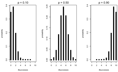
Fig. 1 Three binomial probability mass functions with n = 10 and p = 0.1, 0.5, and 0.9
Observe that as p approaches the endpoint values of 0 and 1 the distributions are more skewed. When p = 0.5 the distribution looks quite symmetric. I repeat this for p = 0.5, 0.8, and 0.9 but this time with a much larger number of trials, n = 100.
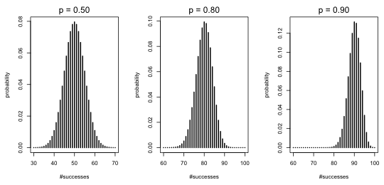
Fig. 2 Three binomial probability mass functions with n = 100 and p = 0.5, 0.8, and 0.9
Notice that the distributions for p = 0.5 and 0.8 are nearly perfectly symmetrical, while the distribution for p = 0.9 is nearly symmetrical showing only a hint of left skewness.
Because a binomial distribution is the sum of n independent Bernoulli random variables, the central limit theorem applies. According to the central limit theorem when we add up a large number of independent and identically distributed random variables, no matter what their distribution, the sum will tend to look normally distributed. Fig. 2 is an illustration of the central limit theorem in practice and is an empirical rationale for using a normal distribution to approximate the binomial. Practically speaking, if you have binomial data and your n is big enough, you could analyze your binomial counts as if they came from a normal distribution. In order for the approximation to be good the recommendation is that both the products np and n(1–p) need to be large. If both products exceed 5 that is typically large enough for the normal approximation to be a reasonable one.
To illustrate constructing the likelihood of a binomial random variable we consider a seed germination experiment in which 100 seeds are planted in a pot and the number of seeds that germinate is recorded. Suppose this is done repeatedly for different pots of seeds such that the different pots are each subjected to different light regimes, burial depths, etc. Clearly the first two assumptions of the binomial distribution hold here.
Assumptions (3) and (4), constant p and independent trials, would need to be verified. Suppose there are m pots subjected to different treatments and in each pot we record the total number of germinated seeds. Let the probability of germination in pot i be pi and to make things more general suppose ni seeds were planted in pot i. We make the usual assumption that the outcomes in different pots are independent of each other. Then we can write the down the following likelihood for our model.
Except for the leading product of binomial coefficients the remainder of the likelihood looks just like the likelihood of the product Bernoulli model. The only real substantive difference is that in the binomial model the probabilities p are the same for observations coming from the same group (pot) whereas in the product Bernoulli model all the probabilities are potentially different. As a result when we formulate a regression model for binomial data our predictors will vary for different groups (pots) but will be constant for all the Bernoulli trials that make up a group. In contrast to this in the product Bernoulli model each individual binary observation can have a different values of a predictor.
Because the binomial distribution assumes that each binomial outcome arises from a sequence of independent Bernoulli trials, a binomial experiment with m binomial random variables each constructed from n independent Bernoulli trials yields a likelihood consisting of a product of m × n Bernoulli probabilities. This is exactly what we would obtain if we had used a product Bernoulli model and viewed the experiment as consisting of m × n independent ordered Bernoulli trials. The likelihoods differ only in the presence of the binomial coefficients.
Because the binomial coefficients in the binomial likelihood don't contain p, they do not affect our estimate of p. So, whether we treat a binomial experiment as grouped binary data or ordered binary data we will obtain the same maximum likelihood estimates of the parameters. Because the likelihood of the binomial model also contains the binomial coefficients the reported log-likelihoods at the maximum likelihood estimates will differ between the two approaches (as will the residual deviance and the AIC), but the estimates, their standard errors, and significance tests will all be the same.
With continuous data our basic regression model took the following form.
With count data our basic regression model took the following form.
(A model similar to this was used for the negative binomial distribution.) The use of the log link with count data is important because it guarantees that the mean of the Poisson (negative binomial) distribution will be greater than zero. A potential down side is that while the predictors act additively on the log mean scale they will act in a multiplicative fashion on the mean on the original scale of the response.
Fitting regression models using a binomial distribution poses an additional challenge. The parameter p that we wish to model is bounded on two sides. It is bounded below by zero and above by one. Thus in order for the regression model to yield sensible results we need a link function that will constrain p to lie within these limits. The most popular modern choice for such a link function is the logit function. Thus with binary data the basic logistic regression model takes the following form.
The logit, also called a log odds, is defined as follows.
"Odds" is meant in the sense that a gambler uses the term odds. In truth the concept of "odds" is completely interchangeable with the concept of probability. If you're told that the probability of a success is ![]() that translates into saying that the odds are 2 to 1.
that translates into saying that the odds are 2 to 1.
If on the other hand you're told that the odds are 1.5 in favor of an event this means that the probability of a success is ![]() .
.
So, odds are an equivalent although perhaps less familiar way of talking about probability. Odds can be any number from 0 to ∞. Taking the log of the odds then can yield any number on the real line. So, the logit maps a probability, a number in the open interval (0, 1), onto the set of real numbers. The benefit of using a logit link in binary regression is that it permits the regression equation to take on any value (negative or positive) while guaranteeing that when we back-transform the logit to obtain p, the result will lie in the interval (0, 1).
Although the logit is the most popular link function for binomial data because of its interpretability as a log odds, there are other possible choices for the link function. Historically a commonly used alternative was the probit function defined to be ![]() where Φ is the cumulative distribution function of the standard normal distribution. Because
where Φ is the cumulative distribution function of the standard normal distribution. Because ![]() the function Φ maps real numbers into the interval [0, 1]. The probit, being the inverse function, therefore maps probabilities onto the real line. By inverting the probit function we can obtain a probability corresponding to a probit regression prediction. For binomial data the glm function of R offers the logit link (the default), the probit link, and a third link called the complementary log log (cloglog) link.
the function Φ maps real numbers into the interval [0, 1]. The probit, being the inverse function, therefore maps probabilities onto the real line. By inverting the probit function we can obtain a probability corresponding to a probit regression prediction. For binomial data the glm function of R offers the logit link (the default), the probit link, and a third link called the complementary log log (cloglog) link.
Although Poisson data resemble binomial data they are fundamentally different. Poisson counts are unbounded above, while binomial counts are bounded above by n. As a result we always know that a binomial response cannot exceed n, the total number of trials, whereas a Poisson response theoretically has no upper bound.
As an example the bycatch data from Assignment 10 that we analyzed using Poisson regression superficially looks like binomial data. The response variable was the number of dolphins caught over a fixed number of tows for each trip. The difference is that we weren't treating the outcome of each tow as a success or a failure. We just counted up the number of dolphins caught, so the individual tows were not Bernoulli trials. On a single tow there could be many dolphins caught, one dolphin, or none. So, potentially at least, there was no maximum value for the number of dolphins caught; the number could conceivably exceed the number of tows. We did include the number of tows in the model as a covariate (or an offset) to account for the fact that the observations in the data set were not equivalent because they were obtained with unequal degrees of effort.
Still, there are situations where it is legitimate to treat binomial data as having an approximate Poisson distribution. The classical instance of this is a binomial experiment in which n is extremely large and p is extremely small. In this case if we let λ = np and calculate probabilities P(X = k) using a Poisson or a binomial model, the answers we get are very similar.
There is a formal theorem that specifies the conditions for which a Poisson distribution can be viewed as the limiting case of a binomial distribution.
The data set for today's lecture is taken from Piegorsch and Bailer (2005) who describe it as follows (p. 126).
In the late 1980s, the US Geological Survey (USGS) conducted a water quality study of land on Long Island, New York (Eckhardt et al., 1989). As part of the study, results were presented on contamination of the groundwater by the industrial solvent trichloroethylene (TCE). We have Y = number of wells where TCE was detected, out of N sampled wells in total. Also recorded for use as potential predictor variables were the qualitative variables xi1 = land use (with 10 different categories), and xi2 = whether or not sewers were used in the area around the well, along with the quantitative variates xi3 = median concentration (mg/L) of nitrate at the N well sites, and xi4 = median concentration (mg/L) of chloride at the N well sites. Interest existed in identifying if and how these predictor variables affect TCE contamination.
I load and examine the data.
Each row is a single binomial observation, the observed number of successes y out of a fixed total n. An observation is classified as a "success" if the well is contaminated with TCE. The binomial distribution has two parameters, n and p. We are given n for each observation but we need to estimate p, the probability of success. Our goal is to quantify how p depends on the measured predictors: land use (categorical), sewer use (categorical), nitrate (continuous), and chloride (continuous). The land use categories are: undeveloped (undev), agriculture (agri), low-density residential with less than 2 dwellings/acre (resL), medium-density residential with 2-4 dwellings/acre (resM), high-density residential with greater than 4 dwellings/acre (resH), recreation (recr), institution (inst), transportation (trans), commercial (comm), and industrial (indus).
The source of the binomial grouping for these data is unclear. It is possible that a map of Long Island was stratified into areal regions according to land use (and perhaps the presence of sewers) and then within each stratum a certain number of wells were tested. If this description is correct then we do not have a random sample of wells. Land use and sewer are stratum characteristics that are then inherited by all the wells in that stratum. From the description of the study, chloride and nitrate concentration were measured separately for each individual well but the value reported in the data set is the median value of these concentrations for all the wells in the stratum. Thus for better or worse all of the predictors in the data set are measured at the stratum level, i.e., at the level of the binomial observation (not at the level of the individual well). It's probably the case that these are really binary data (measurements on individual wells) that have been categorized for presentation purposes by landscape type and sewer type.
We can get a preliminary sense of the importance of the categorical predictors sewer and land use with a dot plot of the raw success probabilities for each category.
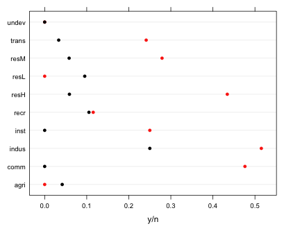
Fig. 3 The effect of sewer and land use on the proportion of contaminated wells
From the graph we see that while there are small differences with respect to land type there are some large effects associated with the presence (red) or absence (black) of sewers.
Logistic regression models are fit in R using the glm function with the argument family=binomial. The logit link is the default and doesn't have to be specified. For true binomial (grouped binary) data the response "variable" is a matrix constructed with the cbind function in which the first column is the number of successes and the second column is the number of failures. I start by fitting an additive logistic regression model that includes only the two categorical variables as predictors.
Deviance Residuals:
Min 1Q Median 3Q Max
-1.5363685 -0.9860019 -0.0001991 0.3541879 1.4394048
Coefficients:
Estimate Std. Error z value Pr(>|z|)
(Intercept) -3.6568 0.7376 -4.957 7.14e-07 ***
land.usecomm 1.8676 0.8044 2.322 0.02025 *
land.useindus 2.2070 0.8053 2.741 0.00613 **
land.useinst 0.7584 0.8395 0.903 0.36629
land.userecr 0.6676 0.8435 0.791 0.42870
land.useresH 1.7316 0.7784 2.225 0.02611 *
land.useresL 0.6663 1.0501 0.635 0.52572
land.useresM 1.0212 0.7809 1.308 0.19099
land.usetrans 0.7933 0.8360 0.949 0.34267
land.useundev -18.3414 3033.9308 -0.006 0.99518
seweryes 1.5980 0.2955 5.407 6.41e-08 ***
---
Signif. codes: 0 ‘***’ 0.001 ‘**’ 0.01 ‘*’ 0.05 ‘.’ 0.1 ‘ ’ 1
(Dispersion parameter for binomial family taken to be 1)
Null deviance: 146.956 on 19 degrees of freedom
Residual deviance: 15.201 on 9 degrees of freedom
AIC: 82.476
Number of Fisher Scoring iterations: 17
Except for the fact that the response is a logit, much of the summary output should look familiar. The land.use and sewer variables are factors and have been entered into the model as dummy variables. The estimates reported in the summary table are for the coefficients of those dummy variables in the model. The coding has been done alphabetically so that the reference group for land.use is agri and the reference group for sewer is sewer = no. As usual then the reported estimates are "effects", the effect of switching from the reference category to the level shown.
Although we haven't discussed ways to interpret the logit, one useful fact about logit(p) is that it is an invertible function that is monotonic in p. Thus when p goes up, the logit goes up; when p goes down, the logit goes down, and vice versa. We can use this fact to interpret how predictors affect the probability that a well is contaminated. Positive coefficients for a dummy regressor mean when we switch from the reference level to the level indicated by the dummy regressor the logit increases. But if the logit increases then the probability of contamination must also increase. Thus we can see from the reported estimates that for all of the land use categories except "undeveloped" the probability of a well being contaminated by TCE is higher for that land use than it is for agricultural land (the reference category), although only some of these differences are significant. Similarly wells on tracts of land that have sewers have a higher probability of being contaminated than do wells on tracts without sewers.
As was pointed out above, the likelihoods for grouped binary data (under a binomial model) and binary data (under a product Bernoulli model) take the same form and yield the same maximum likelihood estimates for the regression parameters. We can demonstrate this by converting the binomial data of the wells data set to binary data. As binary data each observation should generate wells$y ones and wells$n – wells$y zeros. I write a function that generates the zeros and ones on a per observation basis treating a row of the wells data frame as a vector.
I try the function out on the first four observations of the data set using the apply function. The apply function returns a list because the vectors of zeros and ones created from different rows are of different lengths.
$`2`
[1] 0 0 0 0 0 0 0 0 0 0 0 0 0 0 0 0 0 0 0 0 0 0 0 0 0 0 0 0 0 0 0 0 0 0 0 0
[37] 0 0 0 0 0 0 0 0 0 0 0 0 0 0 0 0 0 0 0 0 0 0 0
$`3`
[1] 0 0 0 0 0 0 0
$`4`
[1] 1 1 0 0 0 0 0 0 0 0 0 0 0 0 0 0 0 0 0 0 0 0 0 0 0 0 0 0 0 0 0 0 0 0 0 0
[37] 0 0 0 0 0 0 0 0 0 0 0 0
Finally I do this for all the observations, unlist the results, and add columns indicating the values of the land.use and sewer variables repeated the necessary number of times.
To fit a logistic regression model to binary data we just enter the binary variable as the response and specify the family argument as binomial.
Deviance Residuals:
Min 1Q Median 3Q Max
-1.2409 -0.6666 -0.3332 -0.0001 2.7138
Coefficients:
Estimate Std. Error z value Pr(>|z|)
(Intercept) -3.657 0.738 -4.96 7.1e-07 ***
land.usecomm 1.868 0.804 2.32 0.0203 *
land.useindus 2.207 0.805 2.74 0.0061 **
land.useinst 0.758 0.839 0.90 0.3663
land.userecr 0.668 0.844 0.79 0.4287
land.useresH 1.732 0.778 2.22 0.0261 *
land.useresL 0.666 1.050 0.63 0.5257
land.useresM 1.021 0.781 1.31 0.1910
land.usetrans 0.793 0.836 0.95 0.3427
land.useundev -15.456 716.838 -0.02 0.9828
seweryes 1.598 0.296 5.41 6.4e-08 ***
---
Signif. codes: 0 ‘***’ 0.001 ‘**’ 0.01 ‘*’ 0.05 ‘.’ 0.1 ‘ ’ 1
(Dispersion parameter for binomial family taken to be 1)
Null deviance: 615.83 on 649 degrees of freedom
Residual deviance: 484.08 on 639 degrees of freedom
AIC: 506.1
Number of Fisher Scoring iterations: 17
If you compare this output with the output from the grouped binary data model above, you'll see that the coefficient estimates, standard errors, and p-values are exactly the same (except for the undeveloped land use type, discussed further below). The AIC, log-likelihood, and residual deviance are all different.
So in terms of obtaining estimates and carrying out statistical tests, it doesn't matter whether we view the response as binomial or binary.
It is sometimes useful to see the actual estimates for each category, rather than the estimated effects. We could obtain these estimates by hand by adding the estimate of the intercept to each estimated effect. To obtain standard errors we would need to use the method described in lecture 4. An easier way when it's possible is to refit the model without an intercept. This allows us to see the individual category estimates for one of the factors in the model, namely the factor variable that is listed first in the model formula.
Deviance Residuals:
Min 1Q Median 3Q Max
-1.5363685 -0.9860019 -0.0001991 0.3541879 1.4394048
Coefficients:
Estimate Std. Error z value Pr(>|z|)
land.useagri -3.6568 0.7376 -4.957 7.14e-07 ***
land.usecomm -1.7892 0.4041 -4.427 9.54e-06 ***
land.useindus -1.4498 0.3971 -3.651 0.000261 ***
land.useinst -2.8984 0.4636 -6.252 4.05e-10 ***
land.userecr -2.9892 0.4620 -6.470 9.82e-11 ***
land.useresH -1.9253 0.3478 -5.536 3.10e-08 ***
land.useresL -2.9905 0.7669 -3.899 9.65e-05 ***
land.useresM -2.6357 0.3246 -8.120 4.68e-16 ***
land.usetrans -2.8635 0.4524 -6.329 2.47e-10 ***
land.useundev -21.9983 3033.9307 -0.007 0.994215
seweryes 1.5980 0.2955 5.407 6.41e-08 ***
---
Signif. codes: 0 ‘***’ 0.001 ‘**’ 0.01 ‘*’ 0.05 ‘.’ 0.1 ‘ ’ 1
(Dispersion parameter for binomial family taken to be 1)
Null deviance: 432.213 on 20 degrees of freedom
Residual deviance: 15.201 on 9 degrees of freedom
AIC: 82.476
Number of Fisher Scoring iterations: 17
Observe that land.use = 'agri' has the value of the intercept from the previous model and all of the other land use categories have the old intercept value added to them. These are the predicted logits for each land.use type when sewer='no'. The estimate of sewer is still an effect estimate and is the difference in logits between sewer = 'no' and sewer = 'yes'. If we wanted to see the estimated logits for both sewer categories we would need to list sewer before land.use in the model formula. Removing the intercept has no effect on model fit. The reported AIC values are the same.
The reported standard error for land.use = undev is crazy in all versions of the logistic regression model we've fit. The estimated logit for the undeveloped land use category is –22 with a standard error of 3000 yielding a p-value of 1. This indicates that glm failed to estimate this parameter. If we look at the raw data we can see why this has happened.
Both binomial observations in the undeveloped land use category had 0 successes, i.e., no contaminated wells. This is the only land use category for which this happened. We can get information about successes and failures for each land use category with the xtabs function. xtabs tabulates data by a categorical variable using the value of another variable for the frequencies.
With no successes the maximum likelihood estimate of the probability of success for this category should be zero. This also corresponds to an odds of zero. Because the log of zero is undefined, the logit is undefined for this group thus leading to estimation problems in a logit model. The problem described here is called quasi-complete separation and occurs any time a parameter in a model corresponds to a set of observations that are all successes or all failures. While this is a nuisance when fitting a logistic regression model it is obviously not a bad problem to have. What it means here is that wells on undeveloped land are never contaminated regardless of their sewer status. As a result knowing that land.use = 'undev' perfectly predicts that a well is not contaminated. Unfortunately maximum likelihood estimation has failed as indicated by the ridiculously large standard error reported in the summary table.
When binomial data exhibit quasi-complete separation we have a number of options.
There are alternatives to maximum likelihood estimation when the data are sparse: exact methods (Mehta and Patel 1995; Venkataraman and Ananthanarayanan 2008), a Bayesian approach with an informative prior (Gelman et al. 2008), and the Firth bias reduction method (Firth 1993) that maximizes a penalized likelihood function. The exact approach is proprietary and is only implemented in SAS and logXact. Furthermore the exact method can fail for complicated models. The R package elrm approximates exact logistic regression using MCMC but I’ve found its performance to be somewhat unsatisfactory.
Firth regression is identical to Bayesian logistic regression with a noninformative Jeffreys prior (Fijorek and Sokolowski 2012). Heinze and Schemper (2002) have shown that the Firth method is a general solution to the problem of complete separation. The logistf package of R (Ploner et al. 2010) carries out the Firth method. An extension of the Firth method to multinomial models is implemented in the pmlr package of R (Colby et al. 2010).
The logistf function of the logistf package requires a binary response variable in which the categories have the numerical values 0 and 1. The wells.raw data frame we created previously will work here.
coef se(coef) lower 0.95 upper 0.95 Chisq p
(Intercept) -3.424344 0.670564 -5.025055 -2.313637 68.763252 1.11022e-16
land.usecomm 1.682935 0.744342 0.377902 3.376933 6.695309 9.66669e-03
land.useindus 2.015201 0.745245 0.708822 3.710398 9.935773 1.62097e-03
land.useinst 0.613195 0.778832 -0.793258 2.349624 0.680935 4.09265e-01
land.userecr 0.528785 0.781638 -0.891240 2.267772 0.496065 4.81234e-01
land.useresH 1.545687 0.716133 0.308640 3.201830 6.298950 1.20810e-02
land.useresL 0.654184 0.963398 -1.303080 2.610622 0.469950 4.93010e-01
land.useresM 0.844285 0.718005 -0.401195 2.502388 1.652675 1.98595e-01
land.usetrans 0.646981 0.774896 -0.751044 2.377972 0.769544 3.80358e-01
land.useundev -2.208163 1.578255 -7.148982 0.345864 2.806710 9.38707e-02
seweryes 1.555010 0.286769 1.004491 2.147990 33.464284 7.25847e-09
Likelihood ratio test=124.958 on 10 df, p=0, n=650
The reported estimate and standard error for the undeveloped land use category effect are sensible. According to the output we see that although undeveloped land has a lower probability of well contamination than does agricultural land, the difference is not significant (p = 0.09).What if we had chosen to remove land.use="undev" from the analysis? What should we report as the estimate for this group? Based on the data alone the obvious estimate for the probability of contamination is zero, but what about a confidence interval for this estimate? Do we really believe that there are no contaminated wells on undeveloped land? How should we quantify our uncertainty when we have a point estimate of zero? To understand how to proceed I start with a less severe situation that I then generalize to the case of zero successes.
There were 76 wells tested for land.use='undev'. Suppose we had observed 2 contaminated wells among these 76. The obvious point estimate of the probability of contamination is ![]() . What should we report for a confidence interval? Statistical theory tells us that the variance of a binomial proportion p when the number of trials is n is the following.
. What should we report for a confidence interval? Statistical theory tells us that the variance of a binomial proportion p when the number of trials is n is the following.
Binomial proportions are in principal sums; hence the central limit theorem apples to them and we expect them to be approximately normally distributed when samples are large. A large sample confidence interval for a proportion is the following.
If we use this formula when the success rate is 2 out of 76, we get a silly confidence interval estimate for p.
An interval estimate for a proportion that includes negative values is obviously nonsensical. The usual seat of the pants rule for when the central limit theorem is applicable to proportions is that both np ≥ 5 and n(1 – p) ≥ 5. In our case np = 2 so the guidelines aren't satisfied. One "fix" is to instead assume normality on a logit scale. While this would yield a sensible confidence interval for the current example, it is of no help in dealing with p = 0 because the logit when p = 0 is undefined.
Another solution is to construct what's called an exact confidence interval. It's called exact because it is based not on a normal approximation but instead on the exact tail probabilities of the binomial distribution. The idea is simple. Let the desired confidence interval for p be denoted ![]() and consider the case where we observe X = 2 successes out of n = 76 trials.
and consider the case where we observe X = 2 successes out of n = 76 trials.
Fig. 4 displays the two binomial distributions corresponding to pU and pL.
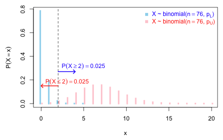
Fig. 4 Finding an exact confidence interval for p when X ~ binomial(n = 76, p) R code
It's not hard to obtain pU and pL iteratively by starting with an initial guess and then refining it. To find pU I just keep trying new values for pU such that pbinom(2,size=76,p=pU) gets as close as possible to 0.025.
To find pL we use the fact that P(X ≥ 2) = P(X > 1) = 1 – P(X ≤ 1) = 1-pbinom(1, size=76, p=pL).
So, an approximate answer is (.0032, .0918). But there's no need to do this by hand. The binom.test function of R will generate this very same confidence interval.
data: 2 and 76
number of successes = 2, number of trials = 76, p-value < 2.2e-16
alternative hypothesis: true probability of success is not equal to 0.5
95 percent confidence interval:
0.003203005 0.091849523
sample estimates:
probability of success
0.02631579
The interval that we've calculated is called the Clopper-Pearson interval. A number of other kinds of confidence intervals are available for proportions. See, e.g., Agresti (2002), p. 14–21, and Brown et al. (2001). What about the the case when there are 0 successes? Here's what the binom.test function reports.
data: 0 and 76
number of successes = 0, number of trials = 76, p-value < 2.2e-16
alternative hypothesis: true probability of success is not equal to 0.5
95 percent confidence interval:
0.00000000 0.04737875
sample estimates:
probability of success
0
The 95% confidence interval is (0.000, 0.047). The convention is to take 0 as the lower limit when zero successes are observed, but the upper limit is calculated in the manner that was just described.
We can combine the undeveloped land use category with another similar category (either theoretically similar or empirically similar) and refit the model. A priori it would make sense to combine it with some other low impact category. Using the individual logit estimates from glm or the empirical probability estimates shown below, it would appear that the undeveloped category is most similar to the agriculture category.
I combine these two categories to make a new land use category and then refit the model with the new land use variable. For the moment I continue to fit a model without an intercept so that I can compare the logits corresponding to the different land use categories.
Deviance Residuals:
Min 1Q Median 3Q Max
-1.5494 -1.0623 -0.3001 0.3583 1.7330
Coefficients:
Estimate Std. Error z value Pr(>|z|)
land.use2comm -1.7699 0.4027 -4.395 1.11e-05 ***
land.use2indus -1.4328 0.3956 -3.621 0.000293 ***
land.use2inst -2.8810 0.4622 -6.233 4.58e-10 ***
land.use2recr -2.9745 0.4607 -6.456 1.08e-10 ***
land.use2resH -1.9062 0.3462 -5.507 3.66e-08 ***
land.use2resL -2.9810 0.7660 -3.892 9.96e-05 ***
land.use2resM -2.6230 0.3232 -8.116 4.83e-16 ***
land.use2rural -4.6878 0.7317 -6.407 1.48e-10 ***
land.use2trans -2.8475 0.4511 -6.313 2.74e-10 ***
seweryes 1.5770 0.2937 5.369 7.91e-08 ***
---
Signif. codes: 0 ‘***’ 0.001 ‘**’ 0.01 ‘*’ 0.05 ‘.’ 0.1 ‘ ’ 1
(Dispersion parameter for binomial family taken to be 1)
Null deviance: 432.213 on 20 degrees of freedom
Residual deviance: 19.289 on 10 degrees of freedom
AIC: 84.565
Number of Fisher Scoring iterations: 5
Notice that AIC tells us that this last model is worse than the previous model.
This is an illustration of why AIC should not always be taken seriously. The previous model yielded an estimated logit with a ridiculous standard error for the undeveloped land use category. Although the estimated logit was very negative it was still not significantly different from zero. A logit of zero corresponds to p = 0.50. So even though the point estimate for the probability of contamination for undeveloped land is near zero the very wide confidence interval tells us the true value could be any number between 0 and 1. Reporting the estimates from such a model doesn't make any sense
After collapsing the agricultural and undeveloped land use categories, land use is now a categorical variable with nine levels. Categorical variables with a lot of levels are extremely unwieldy to work with. One approach is to work with the variable as is and then in the end carry out a sequence of post hoc comparisons, such as all pairwise comparisons, to see what's different from what. With 9 categories this would mean 36 different pairwise comparisons of which we'd expect at least two significant results just by chance. After carrying out all these tests we would then be faced with the task of making sense of them.
I find the post hoc testing approach nonsensical, counter-productive, and inconsistent with basic regression modeling strategies. It is also antithetical to the information-theoretic approach to model selection that is very popular in the biological literature (lecture 19). In keeping with the information-theoretic approach I propose that we should make the re-categorization of the land use variable a part of the model building process itself. To this end I suggest that we fit different models in which the land use variable is categorized in different ways and then use AIC to select the superior categorization. Ideally the re-categorization should be done on theoretical grounds. For instance if we think intensity of land use drives well contamination with TCE then we could try a re-categorization that combines land use categories based on some measure of intensity. Because I don't have any theory to work with here I'm going to use a data-snooping empirical approach. I combine land use categories based on the similarities of their estimated logits. To facilitate this I plot the nine estimated land use logits in a single dot plot.
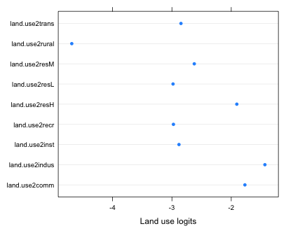
Fig. 5 The predicted logits for different categories of land use
Without worrying about what's significantly different from what, it's pretty clear that the logits fall into three groups. The rural category stands alone but then there are five categories all with logits around –3 and three categories with logits that are larger than –2. These last three all seem to represent high intensity land use: commercial, industrial, and high-density residential. The other five perhaps represent an intermediate level of use intensity. I fit the re-categorization models in stages. First I combine the five middle categories.
AIC argues for the simpler model. Observe that the log-likelihoods of the two models are barely different. If we were to carry out a likelihood ratio test (legitimate here because the two models are nested) we would fail to find a significant difference.
Model 1: cbind(y, n - y) ~ land.use3 + sewer - 1
Model 2: cbind(y, n - y) ~ land.use2 + sewer - 1
Resid. Df Resid. Dev Df Deviance P(>|Chi|)
1 14 20.004
2 10 19.289 4 0.71526 0.9494
The summary table of this last model suggests that the three estimated logits from the high intensity use categories are not very different ranging from –1.4 to –1.9. I proceed to combine them into a single category.
AIC chooses the simplest model with just three land use categories. A likelihood ratio test agrees.
Model 1: cbind(y, n - y) ~ land.use4 + sewer - 1
Model 2: cbind(y, n - y) ~ land.use3 + sewer - 1
Resid. Df Resid. Dev Df Deviance P(>|Chi|)
1 16 21.502
2 14 20.004 2 1.4978 0.4729
Finally I refit this model without an intercept to obtain the estimated logits of the individual land use categories and their confidence intervals.
As a final test of model adequacy I try adding an interaction between land use and sewer.
Model 1: cbind(y, n - y) ~ land.use4 + sewer
Model 2: cbind(y, n - y) ~ land.use4 * sewer
Resid. Df Resid. Dev Df Deviance P(>|Chi|)
1 16 21.502
2 14 18.081 2 3.4206 0.1808
The interaction term is not significant so we can stay with the main effects model. We come to the same conclusion if we use AIC to select the final model.
A compact collection of all the R code displayed in this document appears here.
| Jack Weiss Phone: (919) 962-5930 E-Mail: jack_weiss@unc.edu Address: Curriculum for the Environment and Ecology, Box 3275, University of North Carolina, Chapel Hill, 27599 Copyright © 2012 Last Revised--November 30, 2012 URL: https://sakai.unc.edu/access/content/group/3d1eb92e-7848-4f55-90c3-7c72a54e7e43/public/docs/lectures/lecture26.htm |