Lecture 14—Wednesday, October 10, 2012

Topics

• Poisson distribution
  • Basic characteristics
  • Probability mass function for the Poisson
  • Importance and use
  • Theoretical motivation for the Poisson distribution
  • Examples of Poisson distributions
• Traditional strategies for analyzing count data
• Poisson model for aphid counts
  • Constructing the Poisson log-likelihood
  • Graphing the log-likelihood
  • Maximizing the log-likelihood numerically
• Cited references

R functions and commands demonstrated

• barplot is the base graphics function for generating bar plots.
• dpois is the probability mass function of the Poisson distribution.
• mtext adds text to the margin of a graph.
• nlm is the nonlinear minimization function of R.
• prod calculates the product of all the elements of a vector.

R function options

• hessian= (argument to nlm) can be assigned the values TRUE or FALSE (the default). When TRUE the Hessian is reported evaluated at the minimum value obtained by nlm.
• line= (argument to mtext) specifies how far away (in line units) from the plot border to add the text.
• mfrow= (argument to par) divides the graphics window into a specified number of rows and columns.
• side= (argument to mtext) specifies the side of the graph on which to place the text: 1 = bottom, 2 = left, 3 = top, 4 = right.
• type= (argument to plot, points, and lines) controls what is plotted. We used type='h' to drop vertical lines from plotted points.

Poisson Distribution

Basic characteristics

• A Poisson random variable is discrete.
• A typical use for the Poisson distribution is as a model for count data.
• The Poisson distribution is bounded on only one side. It is bounded below by 0, but has no upper limit. This distinguishes it from the binomial distribution which is bounded on both sides.
• Example of a Poisson random variable: the number of cases of Lyme disease in a North Carolina county in a year.
• If the following three assumptions hold then any non-negative discrete random variable recording the number of events in an interval of time or in a region of space will follow a Poisson distribution.
  1. Homogeneity assumption: Events occur at a constant rate λ such that on average for any length of time t we expect to see λt events.
  2. Independence assumption: For any two non-overlapping intervals the number of observed events is independent.
  3. If the interval is very small, then the probability of observing two or more events in that interval is essentially zero. (More specifically, this probability is much, much smaller than the probability of observing one event.)
• The Poisson distribution is a one-parameter distribution. The parameter is usually denoted with the symbol λ, the rate.
• The mean of the Poisson distribution is equal to the rate, λ. The variance of the Poisson distribution is also equal to λ. Thus in the Poisson distribution the variance is equal to the mean. When the mean gets larger, the variance gets larger at exactly the same rate. So we have if then

Mean:

Variance:

• The R Poisson probability functions are dpois, ppois, qpois, and rpois.

Probability mass function for the Poisson

Let where N_t is the number of events occurring in a time interval of length t, then the probability of observing k events in that interval is

The Poisson distribution can be applied to events occurring in time or space. In a Poisson model of two-dimensional space, events occur again at a constant rate such that the number of events observed in an area A is expected on average to be λA. In this case the probability mass function is written as follows.

Often in application the time interval or the area is the same for all observations. For example, if all the quadrats are the same size then we don't need to know what A is. In such cases we suppress t and A in our formula for the probability mass function and write instead

Importance and Use

For spatial distributions the Poisson distribution plays a role in defining a common null model called CSR—complete spatial randomness.

• If we imagine moving a window of fixed size over a landscape then due to the homogeneity assumption of the Poisson distribution, no matter where we move the window the picture should look essentially the same. We will on average see the same number of events in each window. This rules out clumping. If the distribution were aggregated then some snapshots from our moving window would show many events, while others would show none. Note: in a clumped distribution the variance will be greater than the mean.
• Due to the independence assumption the spatial distribution under CSR will not appear very regular. If a regular, equally-spaced distribution is observed then nearby events are interfering with each other to produce the regular spacing. The assumption of the independence of events in non-overlapping regions means that interference of this sort is impossible. In a regular distribution the variance is smaller than the mean.

Theoretical motivation for the Poisson distribution

Many probability distributions have no theoretical motivation but get used in biological applications because they resemble distributions seen in nature. Unlike these distributions the Poisson distribution can be motivated by theory. There are two primary ways that the Poisson distribution arises in practice from theory.

1. Using the three assumptions listed above one can derive the formula for the Poisson probability mass function directly from first principles. The process involves setting up differential equations that describe the probability of seeing a new event in the next time interval. If you would like to see how this is done see this document from a probability for engineers course taught at Duke. This theoretical motivation for the Poisson is important because if a Poisson model does not fit our data it can help us understand why not. We can examine the three assumptions (the first two anyway) and try to determine which one(s) is(are) being violated.
2. Another way the Poisson probability model arises in practice is as an approximation to the binomial distribution. Suppose we have binomial data in which p, the probability of success is very small, and n, the number of trials, is very large. In this case the Poisson distribution is a good approximation to the binomial where λ = np. Formally it can be shown that if you start with the probability mass function for a binomial distribution and let n → ∞ and p → 0 in such a way that np remains constant, you obtain the probability mass function of the Poisson distribution. Here's a document from a physics course taught at the University of Oregon that illustrates the proof of this fact.

Examples of Poisson distributions

I graph the Poisson distribution for different choices of the parameter λ. The argument type='h' drops a vertical line from the plotted point to the x-axis. The mtext function adds text to the margin of a graph. The side argument specifies the edge: 1 = bottom, 2 = left, 3 = top, 4 = right. The line argument specifies the distance from the edge in line units. The mfrow argument of par divides the graphics window into the specified number of rows and columns.

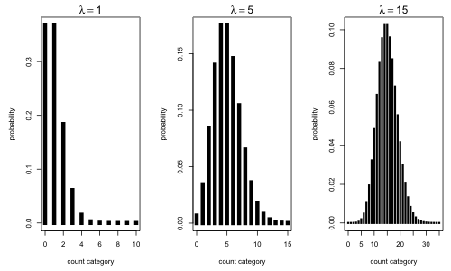
Fig. 1  The Poisson distribution for different choices of the rate constant λ

Notice that when the rate constant λ = 1 the zero category is extremely common comprising nearly 40% of the observations. For small values of λ the Poisson distribution is skewed, but as λ gets larger the Poisson distribution becomes more symmetric. Not surprisingly given that counts are really sums, the central limit theorem kicks in when λ gets large enough (usually λ > 30 is sufficient). In such cases it is reasonable to use a normal distribution to approximate the discrete Poisson distribution if desired. Keep in mind that in using the normal distribution it will be necessary to calculate probabilities over intervals to find the probabilities of specific count categories. For example, using a normal distribution we would have to calculate the Poisson probability P(X = 16) as follows.

In Fig. 1(c), where λ = 15, we could approximate the Poisson probability as follows.

So even with λ = 15 the normal approximation is quite good.

Traditional strategies for analyzing count data

There are a number of standard recommendations for analyzing count data. These date from a time when statistical tools were more limited than they are today. The recommendations are usually some variation of the following. (See, e.g., Snijders and Bosker, 1999, pp. 234–235.)

1. If the counts are all large then standard statistical procedures that assume a normal distribution can be used directly on the raw data. This follows from the fact that count data are essentially sums and the central limit theorem applies to sums when they are large. The term large is relative, but λ > 30 is reasonable although even smaller values of λ will work as long as the the individual counts don't approach the lower boundary of zero.
2. If the counts are only moderately large, say eight or larger, a transformation is advisable. Popular transformations for count data are the square root, logarithm, and Freeman-Tukey transformation. The transformed data can then be used in procedures that assume homoscedastic normally distributed data. It’s worth noting that transformations, by changing the model being fit, lead to additional complications, both in interpretation and in statistical inference. For a critique of the use of data transformations in ecology see McArdle and Anderson (2004).
   1. If there are some zeros along with only moderately large counts the square root is typically recommended.
   2. The logarithm is a more extreme transformation than the square root. If there are some extremely large counts then a log transform may work better. If any of the observed counts are zero then the logarithm is undefined. A common strategy in this case (albeit fraught with problems) is to carry out the transformation log(x + c) where c is a small constant that is added to all the observations x, zero or not. Typically c = 0.5 is chosen without much justification. It is easy to construct cases where the choice of c can markedly change the results (Yamamura 1999).
3. If the data consist of at least some small counts, a discrete probability distribution should be considered as a probability model and the untransformed raw data analyzed directly. For probability distributions such as the Poisson that are in the exponential family a generalized linear model is a popular choice. For other distributions the likelihood needs to be constructed from first principles and worked with directly.

The consensus today is that in cases (1) and (3) a Poisson distribution can be used although in case (1) the Poisson will be nearly indistinguishable from a normal distribution. Case (2) is best handled by assuming a negative binomial distribution for the response rather than transforming the response variable (O’Hara & Kotze 2010). This is especially true if there are both large counts and zeros in the data set. In practice log-transforming and assuming normality or using a negative binomial distribution tend to give nearly identical results, but the negative binomial is better able to handle zero counts and is easier to interpret. Contrary to the nay-sayers like O’Hara & Kotze (2010) there are still cases where you may want to log transform count data and assume normality. The Poisson and especially the negative binomial distribution can be difficult to fit with structured data sets that necessitate the inclusion of random effects. On the other hand these models are relatively easy to fit if one can assume the response is normally distributed.

Poisson model for aphid counts

The data set we'll examine today is shown below. It tabulates the number of aphids found on a random sample of plant stems. It appears on p. 130 of Krebs (1999) but he doesn't give a source for it.

Our goal today is to a fit Poisson distribution to these data. Since the Poisson distribution is a one-parameter distribution with parameter λ the problem reduces to estimating λ. Typically Poisson regression models include predictors in which we make λ a function of those predictors. From a regression standpoint what we're doing today is fitting a Poisson regression model in which the only predictor is an intercept.

The data in Table 1 are given in summary form. The raw data would consist of a list of stems with a count of how many aphids were found on each stem. The table above groups the stems together based on how many aphids were found. The raw data can be recreated from the grouped data with R's rep function. With rep we can repeat the numbers in the first column—0, 1, 3, …, 9—the exact number of times listed in the second column. Recall how rep works. The first argument to rep is what we want to repeat; the second argument describes how the repetition is supposed to be done.

• If the second argument of rep is a single number, then the first argument is repeated that many times as a unit.

  rep(4,10)
  [1] 4 4 4 4 4 4 4 4 4 4
  rep(0:9,4)
   [1] 0 1 2 3 4 5 6 7 8 9 0 1 2 3 4 5 6 7 8 9 0 1 2 3 4 5 6 7 8 9 0 1 2 3 4
  [36] 5 6 7 8 9

• If the second argument is a vector whose length is the same as the length of the first argument, then the elements of the two vectors are matched up 1-to-1. If each element of the vector in the second argument is the same, then the elements of the first argument are all repeated the same number of times, but individually this time, not as a unit.

  rep(0:9, rep(4,10))
   [1] 0 0 0 0 1 1 1 1 2 2 2 2 3 3 3 3 4 4 4 4 5 5 5 5 6 6 6 6 7 7 7 7 8 8 8
  [36] 8 9 9 9 9

  In specifying the repetition pattern for the second argument I used a shortcut. I wrote rep(4,10) which produces, as shown above, a vector of all 4s that is of length 10.

Now we're ready to recreate the data. To do this I make the second argument of rep the observed frequencies shown in the second column of Table 1.

Given that there are no gaps in the count categories, we can visualize the distribution of the tabulated data with a bar chart using the barplot function.

To get labels on the categories we need to add a names attribute to the vector num.stems.

(a)	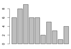(b)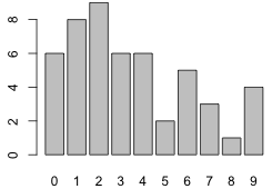
Fig. 2  Bar plots of the tabulated data: (a) without and (b) with the names attribute of the vector

Constructing the Poisson log-likelihood

The first equality follows because we are assuming that we have a random sample and hence the individual observations are independent. Our goal is to fit a Poisson distribution to these data. Once we replace the generic probability expression in the above expression above with a hypothesized probability model, we refer to the new expression as a likelihood. When we take the log of the likelihood we obtain the log-likelihood.

The quantity inside the parentheses is just the dpois function evaluated at x_i and λ. The dpois function is listable. Thus for a fixed value of λ we can obtain the probabilities for all of our observations at once. For example, when λ = 1 we have

Next we need the log of all these values.

Finally we need to sum up all these values.

The last line is what we need for our log-likelihood function. We just need to turn it into a function in which lambda is the sole argument.

The function seems to work.

Graphing the log-likelihood

To graph the log-likelihood, we need to evaluate our function on a whole list of possible values of λ and then plot the results against λ. For example to plot over the range 1 ≤ λ ≤ 6, we could first generate a vector of values for λ in increments of 0.1 with seq(1,6,.1). But when I apply the log-likelihood function to this vector I can see something went wrong.

R returns a single number. I was expecting it to return a list of numbers one for each value of seq(1,6,.1). What if I give it two numbers?

As we can see when I give it both 1 and 2 the answer I get is neither the value at 1 nor the value at 2. To understand what's happening let's tease apart the function into its components. I repeat the above exercise using just the innermost part of our function, dpois.

If you compare the output from the three function calls. you'll see that in the last call R alternates its use of λ = 1 and λ = 2. For the first observation it uses 1, for the second it uses 2, for the third it uses 1, etc. Thus R is trying to match up the entries in each vector argument and when it runs out of entries in the second vector it just recycles the second vector over and over again. Of course when we take the log of the results and then sum everything up we get total gibberish.

The solution is to force R to use each element of the λ vector one at a time. The sapply function will do this.

Now we get the right answer. We're ready to do the plot. To obtain the y-coordinates of the graph we need to use sapply. I specify type='l' in the plot function so that the plotted points are connected by line segments thus generating a curve. I use the xlab and ylab arguments to add labels to the axes.

From the graph it would appear that the log-likelihood takes on its maximum value somewhere in the interval 3 ≤ λ ≤ 4. We obtain the same information if we plot the likelihood instead. The prod function replaces the sum function in the function definition of the likelihood.

(a)	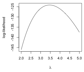(b)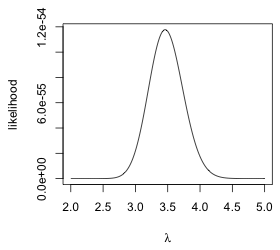
Fig. 3  Plots of the (a) log-likelihood and (b) likelihood functions for a Poisson model for the aphid count data

Maximizing the log-likelihood numerically

We could zoom in on the MLE graphically and obtain an estimate that is as accurate as we please. It can also be shown using calculus that the MLE for λ in a Poisson distribution is the sample mean . Even without this information we can obtain accurate estimates of the MLE using a numerical optimization routine. R provides two numerical optimization functions, nlm and optim, of which I focus on nlm. Figure 4 shows the help screen for nlm.

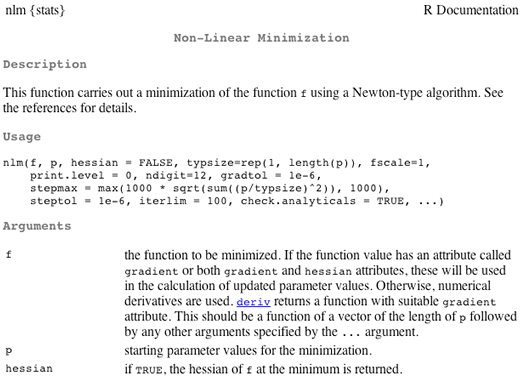
Fig. 4  Help screen for nlm

From the help screen we see that there are only two arguments that are required, f, the function to be minimized, and p, a vector of initial estimates of the parameter values. The rest of the arguments have default values.

Observe that nlm carries out minimization, not maximization. Thus in order for us to be able to use nlm we need to change the way we're formulating our problem. Since maximizing f is equivalent to minimizing –f, we need to reformulate our objective function so that it returns the negative log-likelihood rather than the log-likelihood.

The nlm function uses a method similar to the Newton-Raphson method described in lecture 12. To use nlm we enter the name of our function, poisson.negloglik, as the first argument followed by an initial estimate for its single parameter lambda. Because our graphical analysis indicated that the MLE is near 3, I choose 3 for the initial estimate.

$estimate
[1] 3.459998

$gradient
[1] 6.571497e-08

$code
[1] 1

$iterations
[1] 4

The output tells us the following.

1. The value of the negative log-likelihood at the minimum is 124.1764.
2. The estimate of the MLE of λ is 3.459998.
3. The value of the gradient at the MLE is very small. This is what we want. The gradient is the same as the score, the derivative of the log-likelihood, which from calculus should be zero at a maximum or a minimum. Thus the fact that the value of the gradient is very close to zero encourages us to believe that nlm has found a solution (although there's no guarantee that it's the global minimum that we seek).
4. The help screen tell us that code=1 means "relative gradient is close to zero, current iterate is probably solution."
5. It took 4 iterations of the numerical algorithm to converge.

Using calculus the exact MLE for λ in a Poisson distribution is the sample mean , which turns out to be the same as the estimate returned by nlm.

By adding the argument hessian=T to nlm we can get it to return the value of the Hessian evaluated at the maximum likelihood estimate of λ.

$estimate
[1] 3.459998

$gradient
[1] 1.437515e-07

$hessian
         [,1]
[1,] 14.44799

$code
[1] 1

$iterations
[1] 7

Recall that the information of likelihood theory is the negative of the Hessian. Because we've minimizing the negative log-likelihood here the negative sign is already included in the reported Hessian. Thus the information is also 14.448. Likelihood theory tells us that the inverse of the Hessian is the variance of the maximum likelihood estimate.

We can use this to calculate 95% Wald confidence intervals for λ (assuming that the sample size is large enough that we can assume normality for the distribution of the MLE).

So, a 95% confidence interval for λ is (2.94, 3.98).

Cited references

• Krebs, Charles. 1999. Ecological Methodology. Menlo Park, CA: Addison-Wesley.
• McArdle, Brian H. and Marti J. Anderson. 2004. Variance heterogeneity, transformations, and models of species abundance: a cautionary tale. Canadian Journal of Fisheries and Aquatic Sciences 61: 1294–1302.
• O’Hara, Robert B. and D. Johan Kotze. 2010. Do not log-transform count data. Methods in Ecology and Evolution 1: 118–122.
• Snijders, Tom A. B. and Roel J. Bosker. 1999. Multilevel Analysis: An Introduction to Advanced and Multilevel Modeling. London: Sage Publications.
• Yamamura, K. 1999. Transformation using (x + 0.5) to stabilize the variance of populations. Researches on Population Ecology 43: 229–234.

Course Home Page