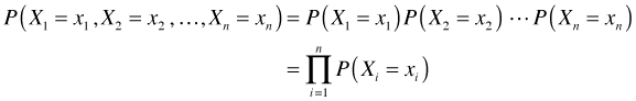
The probability of obtaining a random sample
Let ![]() denote a random sample of size n. We wish to compute the probability of obtaining this particular sample for different probability models in order to help us choose a model. Because the observations in a random sample are independent we can write the generic expression for the probability of obtaining this particular sample as follows.
denote a random sample of size n. We wish to compute the probability of obtaining this particular sample for different probability models in order to help us choose a model. Because the observations in a random sample are independent we can write the generic expression for the probability of obtaining this particular sample as follows.
The likelihood
The next step is to propose a particular probability model for our data. Let![]() denote this probability model where the notation is meant to indicate that the model requires the specification of two parameters α and β. We can replace the generic probability terms in the above expression with the proposed model.
denote this probability model where the notation is meant to indicate that the model requires the specification of two parameters α and β. We can replace the generic probability terms in the above expression with the proposed model.
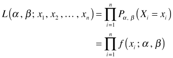
The change in notation on the left hand side is deliberate. The new expression for the probability when treated as a function of α and β is referred to as the likelihood, L, of our data under the proposed probability model.
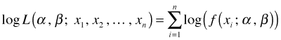
The log-likelihood
Typically we work with the log of this expression now called the log-likelihood of our data under the proposed probability model.
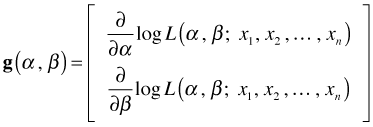
The score (gradient) vector
The maximum likelihood estimates (MLEs) of α and β are those values that make the log-likelihood (and hence the likelihood) as large as possible. The MLEs maximize the likelihood of obtaining the data we obtained. Calculus is used for finding MLEs. The analytical protocol would involve taking the derivative of the log-likelihood with respect to each of the parameters separately, setting the derivatives equal to zero, and solving for the parameters (algebraically when possible, numerically if not). The derivative of the log-likelihood is called the score or gradient vector.
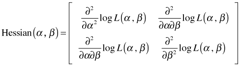
The Hessian
The matrix of second partial derivatives of the log-likelihood is called the Hessian matrix.
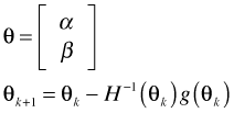
Newton-Raphson method
One method for obtaining maximum likelihood estimates is the Newton-Raphson method. It is an iterative method that makes use of both the gradient vector and the Hessian matrix to update the estimates of the parameters at each step of the algorithm.
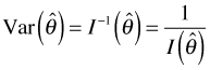
The observed information matrix, I(θ), is is just the negative of the Hessian evaluated at the maximum likelihood estimate. If ![]() is the maximum likelihood estimate of θ based on a sample of size n, then
is the maximum likelihood estimate of θ based on a sample of size n, then
![]()
where ![]() is the inverse of the information matrix (for a sample of size n). Furthermore
is the inverse of the information matrix (for a sample of size n). Furthermore ![]() is asymptotically normally distributed. Thus we have
is asymptotically normally distributed. Thus we have
![]()
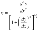
You may have been introduced to the notion of curvature, κ, in your calculus class. The formal definition of the curvature of a curve is the following.

Here φ is the angle of the tangent line to the curve and s is arc length. Thus curvature is the rate at which you turn (in radians per unit distance) as you walk along the curve. For a function written in the form![]() , its curvature can be calculated as follows.
, its curvature can be calculated as follows.
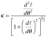
What happens if we apply the curvature formula to the log-likelihood, ![]() ? If the log-likelihood is a function of a single scalar parameter θ, then we have
? If the log-likelihood is a function of a single scalar parameter θ, then we have
Now suppose we evaluate the curvature at the maximum likelihood estimate, ![]() .
.
Recall how the MLE is obtained. We differentiate the log-likelihood and set the derivative equal to zero. Thus, ![]() is the value of θ at which the first derivative of the log-likelihood is equal to zero, i.e.,
is the value of θ at which the first derivative of the log-likelihood is equal to zero, i.e.,
Using this result in the curvature equation above we obtain the following.
Recall that except for the sign, the Hessian (scalar version) at the MLE is what is called the observed information. At the global maximum of a function the second derivative is required to be negative, so taking the negative of the Hessian is just a way of ensuring that the observed information is non-negative. Equivalently we could have taken the absolute value. Thus the observed information is just the magnitude of the curvature of the log-likelihood when the curvature is evaluated at the MLE.
![]()
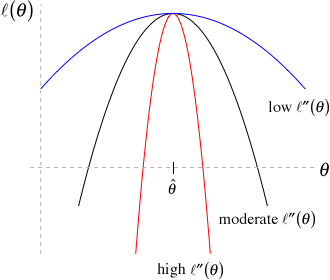
Fig. 1 Curvature and information
A similar argument can be made for a multivariate log-likelihood except that we have multiple directions (corresponding to curves obtained by taking different vertical sections of the log-likelihood surface) to consider when discussing curvature.
So what do these ideas tell us about information in the sense used in likelihood theory? Consider the the graph in Fig. 1 in which three different log-likelihoods are shown. Observe that the three log-likelihoods are all functions of a single parameter θ, they are all maximized at the same place, ![]() , but they have very different curvatures. From red to black to blue we go from high curvature to moderate curvature to low curvature at the maximum likelihood estimate
, but they have very different curvatures. From red to black to blue we go from high curvature to moderate curvature to low curvature at the maximum likelihood estimate ![]() (the value of θ corresponding to the peak of the log-likelihoods). Using the diagram we can make the following observations.
(the value of θ corresponding to the peak of the log-likelihoods). Using the diagram we can make the following observations.
A similar set of statements can be made about the variance of the estimator because for scalar θ the information and the variance are reciprocals of each other.
Using the relationship between information and the variance, we can draw the following conclusions.
The table below summarizes these results more succinctly.
Curvature |
Information |
Confidence interval for θ |
|
high |
high |
low |
narrow |
low |
low |
high |
wide |
The likelihood ratio (LR) test is to likelihood analysis as ANOVA (more properly partial F-tests) is to ordinary linear regression. Partial F-tests are used to compare nested ordinary regression models; likelihood ratio tests are used to compare nested models that were fit using maximum likelihood estimation. Nested models are those that share the same probability generating mechanism, the same response, and all of the same parameters. The only difference is that in one of the models one or more of the parameters are set to specific values (usually zero), while in the other model those same parameters are estimated instead. So we have a restricted model (one in which some parameters are set to specific values) and a second less restricted full model (one in which these same parameters are estimated).
Let θ1 denote the set of estimated parameters from the full model and θ2 denote the set of estimated parameters from the restricted model. Because the models are nested the parameter set θ2 is a subset of the parameter set θ1. The likelihood ratio test takes the following form.
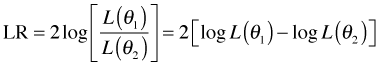
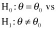
Fig. 2 Geometry of the LR test
It turns out ![]() , a chi-squared distribution with p degrees of freedom, where the degrees of freedom p is the difference in the number of estimated parameters in the two models.
, a chi-squared distribution with p degrees of freedom, where the degrees of freedom p is the difference in the number of estimated parameters in the two models.
Let's consider the special case when there is only a single parameter θ and the restricted model specifies a value for this parameter that we'll denote θ0. (A common case would be θ0 = 0.) Then we have
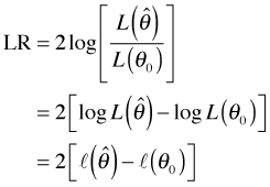
where to simplify notation I use ![]() to denote
to denote ![]() . Fig. 2 illustrates the geometry of the LR test. The LR statistic maps closeness on the θ-axis into closeness on the log-likelihood axis (through the mapping given by the log-likelihood function). In the LR test two values of θ are deemed close only if their log-likelihoods are also found to be close. The chi-squared distribution provides the absolute scale for measuring closeness on the log-likelihood axis.
. Fig. 2 illustrates the geometry of the LR test. The LR statistic maps closeness on the θ-axis into closeness on the log-likelihood axis (through the mapping given by the log-likelihood function). In the LR test two values of θ are deemed close only if their log-likelihoods are also found to be close. The chi-squared distribution provides the absolute scale for measuring closeness on the log-likelihood axis.
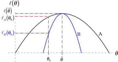
Fig. 3 LR test when the information varies
The role the log-likelihood curve plays in this becomes even clearer when we compare two different log-likelihoods, perhaps arising from different data sets, that yield the same maximum likelihood estimate of θ, but have different curvatures. Fig. 3 illustrates two such log-likelihoods. If we are interested in testing
then scenario B gives us far more information for rejecting the null hypothesis than does scenario A. Observe from Fig. 3 that
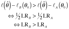
So even though the distance ![]() is the same in both cases, the distances on the log-likelihood scale are different due to their different curvatures. Using the LR test we are far more likely to reject the null hypothesis under scenario B than under scenario A because scenario B provides more information about θ.
is the same in both cases, the distances on the log-likelihood scale are different due to their different curvatures. Using the LR test we are far more likely to reject the null hypothesis under scenario B than under scenario A because scenario B provides more information about θ.
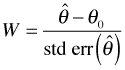
The Wald test is an alternative to the likelihood ratio test that attempts to incorporate the distance ![]() more directly into a test of the null hypothesis
more directly into a test of the null hypothesis
As we've seen in Fig. 3 distance on the θ-axis is not enough. We also need to take into account the curvature of the log-likelihood. In Fig. 3 the more informative scenario B is the one with the greater curvature. In the Wald test we weight the distance on the θ-axis by the curvature of the log-likelihood curves. Formally, the Wald statistic, W, is the following.
where in the second inequality I make use of the relationship between curvature and information that was described above. Taking square roots of both sides yields the Wald statistic.
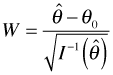
Recall that ![]() . Thus the Wald statistic W can also be written as
. Thus the Wald statistic W can also be written as
From likelihood theory we also know that asymptotically the MLE is unbiased for θ and under the null hypothesis ![]() is the true value of θ. So asymptotically, at least, if the null hypothesis is true then
is the true value of θ. So asymptotically, at least, if the null hypothesis is true then ![]() . Thus asymptotically the expression for W given above is a z-score: a statistic minus its mean divided by its standard error. Since we also know that the MLE of θ is asymptotically normally distributed, it follows that W, being a z-score, must have a standard normal distribution. This provides the basis for the Wald test as well as Wald confidence intervals. (Note: Another way of viewing the Wald test is that it locally approximates the log-likelihood surface with a quadratic function.)
. Thus asymptotically the expression for W given above is a z-score: a statistic minus its mean divided by its standard error. Since we also know that the MLE of θ is asymptotically normally distributed, it follows that W, being a z-score, must have a standard normal distribution. This provides the basis for the Wald test as well as Wald confidence intervals. (Note: Another way of viewing the Wald test is that it locally approximates the log-likelihood surface with a quadratic function.)
In ordinary regression we assume that the response variable has a normal distribution conditional on the values of the predictors in the model. In a simple linear regression model this would be written as follows.
![]()
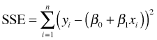
The vertical bar is the usual notation for conditional probability. Thus conditional on the value of x, Y has a normal distribution with mean β0 + β1x and variance σ2. Least squares, which is typically used to obtain estimates of the regression coefficients, makes no assumption about the underlying probability model. Least squares finds the values of β0 and β1 that minimize the error we make when we use the model prediction, β0 + β1xi, instead of the actual data value yi. Formally, least squares minimizes the sum of squared errors, SSE.
So, the normal probability model plays no role in least squares parameter estimation. But having obtained parameter estimates for the data at hand we might wonder how stable those estimates are. What would happen if we went back and collected new data from the same population that gave rise to our first sample? Obviously estimates based on the new sample would be different but how different? To answer this question we need to know how observations vary from sample to sample and for that we need a probability model.
In the least squares formulation of the regression problem, the regression line is treated as a signal contaminated by noise. The signal plus noise view of regression is written as follows.
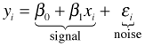
Typically the xi are treated as fixed and the yi and εi are random. Choosing a probability model for εi also gives us a probability model for yi. In the signal plus noise formulation least squares tries to find the values of β0 and β1 that minimize 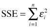 , the sum of the "squared errors". Because the errors are squared, positive and negative deviations from the line are treated as being equally important. Consequently the only reasonable probability distributions for the errors are symmetric ones. This makes the normal distribution an obvious choice. (In the engineering literature various integrated functions of the normal distribution are often referred to as error functions, or erfs.) We assume that
![]()
From this we obtain that the response, yi, is also normally distributed with variance σ2 but with a mean given by the regression line.
Having assumed that the response has a normal distribution, statistical theory tells us that both the intercept and slope will also have normal distributions. This result is the basis for the statistical tests that appear in the summary tables of regression models. Still, it's important to realize that the least squares estimates themselves are obtained without specifying a probability model for the response.
Fig. 1 illustrates the role that the normal distribution plays in ordinary regression. Letting ![]() I generated observations using a model of the form
I generated observations using a model of the form ![]() and used ordinary least squares to estimate the regression line
and used ordinary least squares to estimate the regression line![]() . Fig. 4 displays the raw data used as well as the regression line that was fit to those data.
. Fig. 4 displays the raw data used as well as the regression line that was fit to those data.
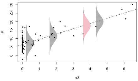
Fig. 4 The normal distribution as a data-generating mechanism. R code for Fig. 4
The estimated errors, ei, are the vertical distances of the individual points to the plotted regression line. The estimated normal error distributions at four different locations are shown. Each normal distribution is centered on the regression line. The data values at these locations are the points that appear to just overlap the bottom edges (left sides) of the individual normal distributions. I've drawn the normal distributions so that they extend ± 3 standard deviations above and below the regression line. (The pink normal curve extends ± 2 standard deviations with the gray tails then extending out the remaining 1 standard deviation.)
Instead of thinking of the normal curves as error distributions, we can think of them as data generating mechanisms. At each point along the regression line, the normal curve centered at that point gives the likely locations of data values for that specific value of x3 according to our model. Recall that 95% of the values of a normal distribution fall within ± 2 standard deviations of the mean while nearly all of the observations (approximately 99.9%) fall within ± 3 standard deviations of the mean. The four selected data values associated with the four displayed normal curves are all well within ± 2 standard deviations of the regression line. Thus they could easily have been generated by the model.
The way to generalize this is obvious. Replace the normal curves by some other probability distribution and think of the new probability models as the data generating mechanisms. How should we choose these probability models? Here are some things to consider when choosing a probability model.
A mathematical function that maps the outcomes of a random experiment (domain) to a set of real numbers (range) is called a random variable. Formally a random variable is a function on the sample space of possible outcomes. Typically in applications the response variable is the random variable whereas the predictors are fixed. If the range of a random variable can be put into one-to-one correspondence with the set of non-negative integers (or if the range is just a finite set) we call the random variable discrete. If the range is the set of real numbers (or a set isomorphic to the set of real numbers) we call it a continuous random variable.
Generally we associate with the random variable X another function called a probability function that describes the probability distribution of X. If X is a discrete random variable we call this function a probability mass function and if X is continuous we call it a probability density function. We will denote the probability function by f(x) or ![]() when we wish to emphasize the fact that the distribution depends on certain parameters that need to be specified. Here the symbols α and β denote the parameters. As an example, in a normal distribution the parameters are the mean μ and the variance σ2.
when we wish to emphasize the fact that the distribution depends on certain parameters that need to be specified. Here the symbols α and β denote the parameters. As an example, in a normal distribution the parameters are the mean μ and the variance σ2.
In an axiomatic formulation of probability theory a probability function must satisfy three properties.
A large number of probability distributions have been studied and been given names. A flowchart of the relationships between those distributions commonly used in scientific applications appears here. A more complete version of this flowchart appears on p. 47 of Leemis and McQueston (2008).
In truth any non-negative portion of a discrete continuous function can be reformulated as a probability function. Consider for instance the function x2, but restricted to the interval 0 ≤ x ≤ 4. If we define
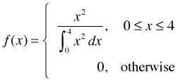
then f(x) satisfies the three properties listed above and hence is a probability density function. Our focus in this course will be on the Poisson, negative binomial, and binomial distributions. Before discussing these we review some of the salient properties of the normal distribution.
The importance of the normal distribution stems from the central limit theorem. In words, if what we observe in nature is the result of adding up lots of independent and identically distributed things, then no matter what their individual distributions are the distribution of the sum tends to become normal the more things we add up. As a practical application sample means tend to have a normal distribution when the sample size is big enough because in calculating a mean we have to add things up.
Even if the response is a discrete random variable such as a count, a normal distribution may be an adequate approximation to its distribution if we’re dealing with a large sample and the values we've obtained are far removed from any boundary values. On the other hand count data with lots of zero values cannot possibly have a normal distribution nor be transformed to approximate normality.
For each probability distribution in R there are four basic probability functions. Each of R's probability functions begins with one of four prefixes—d, p, q, or r—followed by a root name that identifies the probability distribution. For the normal distribution the root name is "norm". The meaning of these prefixes is as follows.
To better understand what these functions do I'll focus on the four probability functions for the normal distribution: dnorm, pnorm, qnorm, and rnorm. Fig. 5 illustrates the relationships among these four functions.
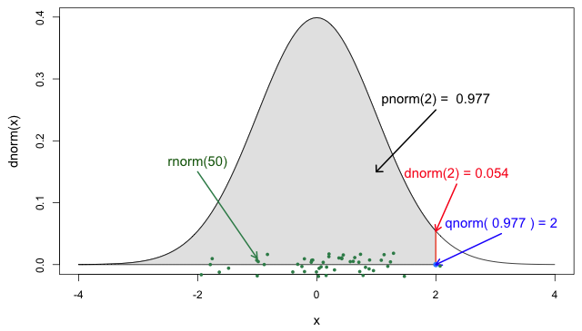
Fig. 5 The four probability functions for the normal distribution R code for Fig. 5
dnorm is the normal probability density function. Without any further arguments it returns the density of the standard normal distribution (mean 0 and standard deviation 1). If you plot dnorm(x) over a range of x-values you obtain the usual bell-shaped curve of the normal distribution. In Fig. 5, the value of dnorm(2) is indicated by the height of the vertical red line segment. It's the y-coordinate of the normal curve when x = 2. Keep in mind that density values are not probabilities. To obtain probabilities from densities one has to integrate the density function over an interval. Alternatively for a very small interval, say one of width Δx, if f(x) is a probability density function, then we can approximate the probability of x being in that interval as follows.
![]()
pnorm is the cumulative distribution function for the normal distribution. By definition pnorm(x) = P(X ≤ x) which is the area under the normal density curve to the left of x. Fig. 5 shows pnorm(2)as the shaded area under the normal density curve to the left of x = 2. As is indicated on the figure, this area is 0.977. So the probability that a standard normal random variable takes on a value less than or equal to 2 is 0.977.
qnorm is the quantile function of the standard normal distribution. If qnorm(x) = k then k is the value such that P(X ≤ k) = x . qnorm is the inverse function for pnorm. From Fig. 5 we have, qnorm(0.977) = qnorm(pnorm(2)) = 2.
rnorm generates random values from a standard normal distribution. The only required argument is a number specifying the number of realizations of a normal random variable to produce. Fig. 5 illustrates rnorm(50), the locations of 50 random realizations from the standard normal distribution, jittered slightly to prevent overlap.
To obtain normal distributions other than the standard normal, all four normal functions support the additional arguments mean and sd for the mean and standard deviation of the normal distribution. For instance, dnorm(x, mean=4, sd=2) is a normal density with mean 4 and standard deviation 2. Notice that R parameterizes the normal distribution in terms of the standard deviation rather than the variance.
| Jack Weiss Phone: (919) 962-5930 E-Mail: jack_weiss@unc.edu Address: Curriculum for the Environment and Ecology, Box 3275, University of North Carolina, Chapel Hill, 27599 Copyright © 2012 Last Revised--October 8, 2012 URL: https://sakai.unc.edu/access/content/group/3d1eb92e-7848-4f55-90c3-7c72a54e7e43/public/docs/lectures/lecture13.htm |