So far in this course we've studied four basic statistical experimental designs: analysis of variance, the randomized block design, analysis of covariance, and the split plot design. As we've seen all of these are just variations of the ordinary regression model. Up until this point we've explicitly assumed a normal distribution for the response variable. We now relax that assumption and turn to situations where the response variable is clearly not normally distributed. We focus especially on instances where the Poisson, negative binomial, or binomial distributions provide better alternatives. To fit regression models to a non-normal response variable requires a different approach to estimation and we consider those methods next.
In statistics we often use a parametric probability model to describe the behavior of a response variable. The role of data in all of this is to provide estimates of the parameters of the probability model. The three most widely-used statistical estimation techniques are
Least squares estimation is extremely popular because it's easy to understand, easy to implement, and has good properties. In simple linear regression the regression model takes the form of deviations about a line:
![]()
The method of least squares obtains values for β0 and β1 that minimize the sum of squared deviations about that line.
The sum of the squared deviations is called the objective function of least squares and it readily generalizes to more complicated scenarios. The standard tools of calculus can used to minimize the objective function and well-defined algorithms exist for finding solutions in both the linear and nonlinear setting. Alternatively the regression problem can be also viewed as vector projection in n-dimensional space for which the standard tools of linear algebra can be applied.
Observe that least squares makes no assumption about an underlying probability model for the response. Typically, a normal model is assumed, but that assumption is tacked on at the end and is not formally part of the least squares solution. A normal probability model is a natural choice for least squares because the basic formulation involving squared deviations necessarily assumes that the errors are symmetrically disposed about the regression surface. Symmetry is also a characteristic of a normal distribution.
For asymmetric probability models, which include most of the ones we'll be discussing in this course, least squares solutions don't make much sense. The two major alternatives to ordinary least squares, maximum likelihood estimation and Bayesian estimation, both incorporate the probability model directly into the objective function rather than tacking it on at the end as an afterthought. We begin with a discussion of maximum likelihood and turn later to Bayesian methods.
We start with the assumption that we have a random sample of size m. For example, suppose we select m shoots at random from a field. On each shoot we count the number of aphids present. The number of aphids observed on a given shoot is a random variable (it has a probability distribution). Denote this random variable by the symbol X. In our random sample then we observe the values of m random variables, X1, X2, ... , Xm, one for each shoot in our sample.
What is the probability of obtaining the data we collected? The notation for this probability is the following.
![]()
This is called a joint probability, the probability of simultaneously observing all m events. (I follow the standard statistical convention of using capital letters for random variables and lower case variables for their values.) Another way of writing this is
![]()
Because we have a random sample, each of these events is independent of the other. From elementary probability theory, if events A and B are independent then we have
![]()
Applying this to our data we have
where I use Π to indicate the product (analogous to Σ for sums).
Now suppose we have a probability model for these data. Later on we'll consider Poisson and negative binomial models for count data, but for the moment we'll treat the probability model generically. Let ![]() denote the probability model. In general f can be a density or a probability mass function where α and β are its parameters. For a Poisson model there is a single parameter, λ, while for a negative binomial model there are two parameters usually denoted μ and θ. When we extend things to include estimating regression models the parameter list will also include the set of regression coefficients in our model. Using this generic probability model we can rewrite the expression for the probability of our data. This new formulation is called the likelihood of our data with respect to the model f.
denote the probability model. In general f can be a density or a probability mass function where α and β are its parameters. For a Poisson model there is a single parameter, λ, while for a negative binomial model there are two parameters usually denoted μ and θ. When we extend things to include estimating regression models the parameter list will also include the set of regression coefficients in our model. Using this generic probability model we can rewrite the expression for the probability of our data. This new formulation is called the likelihood of our data with respect to the model f.
From the likelihood perspective the probability of the data is a function of the parameters α and β. After we've collected the data it's the data that are known and observed while it's the parameter values that are unknown. The likelihood is a probability when we treat the parameters as fixed and the data as random, but when the data are fixed and the parameters are treated as random the likelihood is no longer a probability.
Note: If f is a density function then the likelihood does not derive from a probability. We need to integrate a density in order to obtain a probability. We can get around this "problem" by including an increment ![]() in the expression for the product and then arguing that the product of a density times an increment is an approximation to the true probability.
in the expression for the product and then arguing that the product of a density times an increment is an approximation to the true probability.
For both practical and theoretical reasons, it is preferable to work with the natural logarithm of the likelihood function, i.e., the log-likelihood. For our generic probability model the log-likelihood takes the following form.
In the last step I used a basic property of the logarithm function: for positive numbers a and b, ![]() . So the logarithm function turns multiplication into addition.
. So the logarithm function turns multiplication into addition.
One of R. A. Fisher's many major contributions to statistics was to realize that the likelihood function is a vehicle for obtaining parameter estimates. He proposed what has become known as the maximum likelihood principle for parameter estimation.
Maximum Likelihood Principle: Choose as your estimates of the parameters those values that make obtaining the data that were actually obtained the most probable. In other words, we should choose the parameter values that maximize the value of the likelihood. Typically we maximize the log-likelihood instead of the likelihood.
Another argument in favor of maximum likelihood estimates (MLEs) is that the maximum likelihood estimates of a model's parameters give that model the best chance of fitting the data. If after using these "best" estimates the model is deemed inadequate we can be sure that it is truly inadequate.
Maximizing a log-likelihood can be done in various ways.
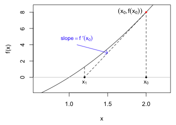
Fig. 1 An illustration of Newton's method (R code)
From calculus we know that all local maxima occur at points where the first derivative is equal to zero, the so-called critical points. In all but the simplest of problems finding a critical point has to be done numerically. Numerical optimization is a rich and active area of research in mathematics, and there are many different approaches available. The Newton-Raphson method is often a good choice.
The Newton-Raphson method is just the multivariate generalization of Newton's method, a method which you should have learned in calculus. Suppose we're trying to find a root of the function f, i.e., the value of x such that f(x) = 0. Fig. 1 illustrates this scenario where it appears that x = 1 is a root of the function f. Newton's method allows us to start with an initial guess for the root and then if our guess is good enough and the function is sufficiently well-behaved, it will after a finite number of steps return a reasonable estimate of the root.
We start with a guess for the root. Fig. 1 shows the guess x0 = 2. We evaluate the function at the guess to obtain the point on the curve labeled (x0, f(x0)). The derivative of f yields a formula for the slope of the tangent line to the curve at any point on the curve. Thus f ′(x0) is the slope of the tangent line to the curve at (x0, f(x0)). A portion of the tangent line is shown in Fig. 1 as the line segment that connects (x0, f(x0)) to the point (x1, 0), the place where the tangent line crosses the x-axis. Using the usual formula for the slope of a line segment we obtain two different expressions for the slope of the displayed tangent line.
I solve this expression for x1 (where at the second step below I assume that ![]() ).
).
Observe from Fig. 1 that x1 is closer to the point where f crosses the x-axis than was our initial guess x0. We could now use x1 as our new initial guess and repeat this process yielding a value x2 that will be closer to the root than was x1.
The formula given above is an example of a recurrence relation and it allows us to use the current value to obtain an updated value. This is the basis of Newton's method. Written more generally the estimate of the root at the (k+1)st step of the algorithm is given in terms of the kth step as follows.
In the maximum likelihood problem we desire the roots of the score function, the derivative of the log-likelihood. To simplify notation let ![]() . Suppose the log-likelihood function is a function of the single parameter θ. Then to find the maximum likelihood estimate of θ we need to find the roots of the equation
. Suppose the log-likelihood function is a function of the single parameter θ. Then to find the maximum likelihood estimate of θ we need to find the roots of the equation

Thus we need the roots of ![]() . In Newton's formula let x = θ,
. In Newton's formula let x = θ, ![]() , and
, and ![]() . Newton's method formula applied to the maximum likelihood problem becomes the following.
. Newton's method formula applied to the maximum likelihood problem becomes the following.
When there are multiple parameters to be estimated θ becomes a vector of parameters, ![]() becomes the gradient or score vector (as was depicted above for two parameters), and
becomes the gradient or score vector (as was depicted above for two parameters), and ![]() becomes a matrix of second partials called the Hessian matrix H. The Hessian matrix when there are two parameters, α and β, is the following.
becomes a matrix of second partials called the Hessian matrix H. The Hessian matrix when there are two parameters, α and β, is the following.
In the formula for Newton's method ![]() occurs in the denominator. This is equivalent to multiplying by its reciprocal. The analogous operation for matrices is matrix inversion. Thus the Newton-Raphson method as implemented for finding the MLEs of a log-likelihood with multiple parameters is the following.
occurs in the denominator. This is equivalent to multiplying by its reciprocal. The analogous operation for matrices is matrix inversion. Thus the Newton-Raphson method as implemented for finding the MLEs of a log-likelihood with multiple parameters is the following.
![]()
Here, for example, θ might be the vector  , g and H are as shown above, and H-1 denotes the inverse of the Hessian matrix.
We've already defined the score function as being the first derivative of the log-likelihood. If there is more than one parameter so that θ is a vector of parameters, then we speak of the score vector whose components are the first partial derivatives of the log-likelihood. As was noted above the matrix of second partial derivatives of the log-likelihood is called the Hessian matrix.
If there is only a single parameter θ, then the Hessian is a scalar function.
The information matrix, I(θ), is an important quantity in likelihood theory. It is defined in terms of the Hessian and comes in two versions: the observed information and the expected information.
which is then evaluated at the maximum likelihood estimate.
The near universal popularity of maximum likelihood estimation derives from the fact that the estimates it produces have good properties. Nearly all of the properties of maximum likelihood estimators are asymptotic, i.e., they only kick in after the sample size is sufficiently large. For small samples there are no guarantees that these properties hold and what constitutes "large" will vary on a case by case basis. In what follows I use the notation ![]() as shorthand for "the maximum likelihood estimate of θ based on a sample of size n."
as shorthand for "the maximum likelihood estimate of θ based on a sample of size n."
This is an abbreviated list because many of the properties of MLEs will not make sense if you don't have the requisite background in statistical theory. Even some of the ones I list here may seem puzzling to you. The most important properties for practitioners are (4) and (5) that give the asymptotic variance and the asymptotic distribution of maximum likelihood estimators.
![]()
Thus the maximum likelihood estimate approaches the population value as sample size increases.
This estimator is biased, which is why we typically use the sample variance as an estimator instead because it is unbiased.
Clearly the difference between these two estimators becomes insignificant as n gets large.
![]()
where
is the inverse of the information matrix (for a sample of size n). This is an important result because it means that the standard error of a maximum likelihood estimator can be calculated.
Properties 2, 4, and 5 together tell us that for large samples the maximum likelihood estimator ![]() of a population parameter θ has an approximate normal distribution with mean θ and variance that can be estimated as
of a population parameter θ has an approximate normal distribution with mean θ and variance that can be estimated as ![]() .
.
![]()
In linear regression we assume ![]() where
where ![]() . If we use maximum likelihood instead of least squares to obtain estimates of β0 and β1 we find that the estimates are identical to the ones we would have obtained using least squares. This happens because the function containing the regression parameters (the sum of squared errors) that is then minimized in ordinary least squares also appears in exactly the same form in the log-likelihood function for this problem. The upstart is that if we use least squares to find the parameter estimates in a regression problem and then assume the errors are normally distributed, or we begin instead by assuming that the response is normally distributed and then use maximum likelihood to estimate the parameters in the regression equation for the mean, we obtain the same results.
. If we use maximum likelihood instead of least squares to obtain estimates of β0 and β1 we find that the estimates are identical to the ones we would have obtained using least squares. This happens because the function containing the regression parameters (the sum of squared errors) that is then minimized in ordinary least squares also appears in exactly the same form in the log-likelihood function for this problem. The upstart is that if we use least squares to find the parameter estimates in a regression problem and then assume the errors are normally distributed, or we begin instead by assuming that the response is normally distributed and then use maximum likelihood to estimate the parameters in the regression equation for the mean, we obtain the same results.
While the estimates of the regression parameters are the same, the maximum likelihood estimate of ![]() is not the same as the one that is typically used in ordinary regression. Just as with the MLE of the sample variance described above, the maximum likelihood estimate of
is not the same as the one that is typically used in ordinary regression. Just as with the MLE of the sample variance described above, the maximum likelihood estimate of ![]() in regression is biased, but the bias does diminish with sample size.
in regression is biased, but the bias does diminish with sample size.
Likelihood theory is one of the few places in statistics where Bayesians and frequentists are in agreement. Both believe that the likelihood is fundamental to statistical inference. They diverge in that frequentists focus solely on the likelihood and use it obtain maximum likelihood estimates of the parameters, while a Bayesian uses it to construct something called the posterior distribution of the parameters.
| Jack Weiss Phone: (919) 962-5930 E-Mail: jack_weiss@unc.edu Address: Curriculum for the Environment and Ecology, Box 3275, University of North Carolina, Chapel Hill, 27599 Copyright © 2012 Last Revised--October 8, 2012 URL: https://sakai.unc.edu/access/content/group/3d1eb92e-7848-4f55-90c3-7c72a54e7e43/public/docs/lectures/lecture12.htm |