In ordinary regression we use ordinary least squares to obtain estimates of the model parameters. If we wish to extend the results beyond the sample at hand, to obtain statistical tests and confidence intervals for the model parameters in the population from which the sample was taken, we need to make an additional assumption about the distribution of the response variable. Typically we assume the response variable has a normal distribution whose mean is given by the regression equation. This assumption can be written as follows.
The first statement is shorthand notation for saying that for observation i the response Y is normally distributed with mean μ and variance σ2. The mean can be different for different observations (and is given by the regression equation) but the variance is the same for all observations. We can combine these two statements and write the simple linear regression model as follows.
![]()
The vertical bar is the usual notation for conditional probability. Thus conditional on the value of x, Y has a normal distribution with mean β0 + β1x and variance σ2.
Having assumed that the response has a normal distribution, statistical theory tells us that both the intercept and slope, when estimated by least squares, will also have normal distributions and we can even derive a formula for their variances. This result becomes the basis for the statistical tests that appear in the summary tables of regression models. Because σ2 is unknown and has to be estimated too, the actual distribution of the regression parameters (at least for small sample sizes) is a t-distribution rather than a normal distribution.
The normality assumption makes possible some new interpretations of the regression model: the signal plus noise interpretation and the data-generating mechanism interpretation.
Least squares makes no assumption about an underlying probability model. Least squares finds the values of β0 and β1 that minimize the error we make when we use the model prediction, β0 + β1xi, instead of the actual data value yi. Formally, least squares minimizes the sum of squared errors, SSE.
The implication from ordinary least squares is that the response variable can be viewed as a signal (the regression line) contaminated by noise. The signal plus noise view of regression can be written as follows.
Typically the xi are viewed as being fixed (measured without error) and only the yi and εi are random. Choosing a probability model for εi automatically gives us a probability model for yi.
According to the signal plus noise formulation least squares tries to find the values of β0 and β1 that minimize  , the sum of the "squared errors". Because the errors are squared, positive and negative deviations from the line are treated as being equally important. Consequently the only reasonable probability distributions for the errors are symmetric ones, making the normal distribution an obvious choice. From the formula for the normal probability density, if the response Yi is normally distributed with variance σ2 and a mean given by the regression line.
![]()
then it follows that the errors are normally distributed with mean 0,
![]()
So a completely equivalent way of writing the normal probability model for the regression problem is the following.
Fig. 1 illustrates a second way of visualizing the role that the normal distribution plays in ordinary regression. Using the signal plus noise interpretation and assuming ![]() I generated observations of the form
I generated observations of the form ![]() and then used ordinary least squares to estimate the regression line
and then used ordinary least squares to estimate the regression line ![]() . Fig. 1 displays the raw data as well as the regression line that was fit to those data.
. Fig. 1 displays the raw data as well as the regression line that was fit to those data.
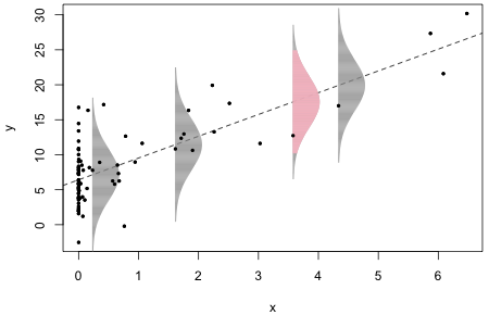
Fig. 1 The normal distribution as a data-generating mechanism. R code for Fig. 1
The estimated normal error distributions at four different locations are shown. Each normal distribution is centered on the regression line. The data values at these locations are the points that appear to just overlap the bottom edges (left sides) of the individual normal distributions. The estimated errors, denoted ei, are the vertical distances of these individual points from the plotted regression line. I've drawn the normal distributions so that they extend ± 3 standard deviations above and below the regression line. (The pink normal curve extends ± 2 standard deviations with the gray tails then extending out the remaining 1 standard deviation.)
Instead of thinking of the normal curves as error distributions, we can think of them as data generating mechanisms. At each point along the regression line in Fig. 1, the normal curve centered at that point gives the likely locations of data values for that specific value of x according to our model. Recall that 95% of the values of a normal distribution fall within ± 2 standard deviations of the mean while nearly all of the observations (approximately 99.9%) fall within ± 3 standard deviations of the mean. The four selected data values associated with the four displayed normal curves are all well within ± 2 standard deviations of the regression line. Thus they could easily have been generated by the model.
When we think of the probability model as a data-generating mechanism, it immediately suggests a way to generalize ordinary linear regression: replace the normal curves by some other probability distribution and think of the new probability models as the data generating mechanisms. On Friday we'll see why we might want to do this for the data set we've been analyzing and starting next week we'll begin this task in earnest.
I refit the various regression models we considered for the rikz data set in lecture 3.
We've seen that statistical tests for the fitted model are displayed in a summary table (obtained using the R summary function on the model) and in an ANOVA table (obtained using the R anova function on the model). We investigate each of these in turn.
The R summary table reports t-statistics and their associated two-tailed hypothesis tests of whether or not a given coefficient is equal to zero. Each test is a regressor added-last test. It compares a regression model with q parameters (where the intercept is one of the q parameters) to a regression model with only q – 1 parameters obtained by dropping the parameter being tested from the model. We start with the summary table for mod1, a model in which NAP is the only predictor of the mean.
![]()
Residuals:
Min 1Q Median 3Q Max
-5.0675 -2.7607 -0.8029 1.3534 13.8723
Coefficients:
Estimate Std. Error t value Pr(>|t|)
(Intercept) 6.6857 0.6578 10.164 5.25e-13 ***
NAP -2.8669 0.6307 -4.545 4.42e-05 ***
---
Signif. codes: 0 ‘***’ 0.001 ‘**’ 0.01 ‘*’ 0.05 ‘.’ 0.1 ‘ ’ 1
Residual standard error: 4.16 on 43 degrees of freedom
Multiple R-squared: 0.3245, Adjusted R-squared: 0.3088
F-statistic: 20.66 on 1 and 43 DF, p-value: 4.418e-05
The highlighted line labeled "NAP" in the summary table tests the following hypothesis about the model.
H0: β1 = 0
H1: β1 ≠ 0
This is a test of whether the mean response is linearly related to NAP. Formally it compares a model with a slope and intercept to a model with only an intercept and tests whether the slope is equal to zero. If we fail to reject this hypothesis then NAP can be dropped from the model.
The line labeled "(Intercept)" in the highlighted output tests the following hypothesis.
H0: β0 = 0
H1: β0 ≠ 0
Formally this compares a model with a slope and an intercept to a model with just a slope (and no intercept, i.e., an intercept = 0) and asks whether we need an intercept. Graphically it tests whether the line passes through the origin. This is usually a useless test. For many data sets the origin is a point outside the range of the data making it just a fitting a constant with no practical interpretation. It turns out for the rikz data set that NAP = 0 is within the range of the data so the test of the intercept here isn't meaningless, but it is still probably uninteresting.
The ANOVA table compares a series of nested models obtained by adding predictors one at a time to a starting model with only an intercept. Predictor here refers to a single variable so if the predictor is a categorical variable represented by dummy regressors in the model, we add the entire set of dummy regressors associated with that categorical variable. Two models are nested if the bigger model (the one with more terms) can be reduced to the smaller model (the one with fewer terms) by setting parameters in the bigger model equal to zero.
R lists the models in an ANOVA table and tests them in a sequential fashion with the simplest model tested listed at the top of the output and the most complicated model listed at the bottom. Tests are based on F-statistics that test whether all the coefficients associated with that predictor are equal to zero. The F-statistic is a ratio: the average amount of variance explained by adding the predictor to the model (model mean squared) divided by the average amount of variance left unexplained (mean squared error) estimated using the most complicated model that was considered. Because the mean squared error is assumed to be just random noise, we are assessing whether the variance reduction obtained by adding the predictor is better than we'd get by chance. Shown below is the ANOVA table for mod1, a model in which NAP is the only predictor.
Response: richness
Df Sum Sq Mean Sq F value Pr(>F)
NAP 1 357.53 357.53 20.66 4.418e-05 ***
Residuals 43 744.12 17.31
---
Signif. codes: 0 ‘***’ 0.001 ‘**’ 0.01 ‘*’ 0.05 ‘.’ 0.1 ‘ ’ 1
Only one model is shown and tested in the output. An additional model not shown is always implicit in these tables and that's a model that contains only an intercept. According to the output the amount of variability that was accounted for by adding NAP to the intercept-only model is 357.53. Since only one parameter was added, the amount of variability explained per parameter added is also 357.53. The amount of variability that remains is given in the line labeled "Residuals" and is reported to be 744.12. This amount of variability is spread out over 43 dimensions, so the average amount of variability is 744.12 divided by 43 or 17.31. If we compare the amount of variability accounted for by the one parameter due to NAP, 357.53, to the average amount of variability remaining, 17.31, the ratio is quite large yielding the reported F-statistic of 20.66. The F-statistic can then be compared to an F-distribution with 1 and 43 degrees of freedom. Based on the reported p-value the F-statistic is statistically significant.
For the simple case of a regression model with a single continuous predictor, the p-value of the F-test and the p-value for the t-test that the slope is equal to zero are exactly the same. The equivalence follows from the mathematical identity
![]()
We can verify this by extracting the t-statistic from the summary table and squaring it. The summary table is stored in the coefficients component of the summary object produced by R. This is a list object and the components can be accessed with the $ notation we've used previously.
We next consider the interaction model mod3 that was fit in R as follows.
Because week is a categorical variable with four levels, it is represented in the regression model with three dummy variables (as was discussed in lecture 2 and lecture 3). The regression model being fit here is the following one.
![]()
The output from the anova function for this model is displayed below. I've added a row number in front of each row of the table for reference.
Response: richness
Df Sum Sq Mean Sq F value Pr(>F)
1 NAP 1 357.53 357.53 59.9605 2.967e-09 ***
2 factor(week) 3 387.11 129.04 21.6406 2.896e-08 ***
3 NAP:factor(week) 3 136.38 45.46 7.6241 0.0004323 ***
Residuals 37 220.62 5.96
---
Signif. codes: 0 ‘***’ 0.001 ‘**’ 0.01 ‘*’ 0.05 ‘.’ 0.1 ‘ ’ 1
There are three different models represented in the table: the interaction model in row 3, the additive model in row 2, and the NAP-only model in row 1. Not shown but used in the reported tests is the intercept-only model. These models form a nested sequence of models with models becoming more complicated as we move down the rows. Models listed lower in the table can be reduced to models listed higher in the table by setting various regression parameters equal to zero.
Tests of whether these reductions should be performed are carried out in rows 3, 2, and 1 of the ANOVA table respectively. Each tests whether the parameters in question are equal to zero versus the alternative that at least one or more of them is not zero. Table 1 summarizes these relationships.
| Table 1 Tests carried out by anova(mod3) |
Row of table |
Model tested |
Terms in model | Test of … | Hypothesis | Model comparison |
– |
mod0 |
1 | overall mean | β0 = 0 | – |
1 |
mod1 |
1 + NAP | NAP | β1 = 0 | mod1 vs mod0 |
2 |
mod2 |
1 + NAP + factor(week) | factor(week) | β2 = β3 = β4 = 0 | mod2 vs mod1 |
3 |
mod3 |
1 + NAP + factor(week) + NAP:factor(week) | NAP:factor(week) | β5 = β6 = β7 = 0 | mod3 vs mod2 |
The anova function can also be used to compare two nested models directly. For example, the third line of the table generated by anova(mod3) can be obtained by comparing models mod3 with mod2 with the anova function.
Model 1: richness ~ NAP + factor(week)
Model 2: richness ~ NAP * factor(week)
Res.Df RSS Df Sum of Sq F Pr(>F)
1 40 357.00
2 37 220.62 3 136.38 7.6241 0.0004323 ***
---
Signif. codes: 0 ‘***’ 0.001 ‘**’ 0.01 ‘*’ 0.05 ‘.’ 0.1 ‘ ’ 1
The test computes the average change in the error sum of squares when the three interaction regressors are added to mod2 and compares it with the average residual squared error in the bigger model mod3. The reported results are identical to what is reported in row three of the output produced by anova(mod3).
Row 3 is the only row of the anova(mod3) output that we can match by comparing two models in this way. When we use the anova function on two nested models it always uses the average residual squared error of the bigger of the two models as the denominator of the F-test, because this is the best estimate of residual noise that it has at its disposal. As a result anova(mod1, mod2) uses the average residual squared error from mod2. On the other hand all the tests carried out by anova(mod3) use the average residual squared error from mod3. As a result the F-statistics we get will be different.
The most sensible way to read the output from anova(mod3) is from the bottom up. Having decided to fit an interaction model at all we should probably test for the presence of an interaction first. If the interaction is significant in mod3 we would carry out no further tests and choose the interaction model as the final model. The usual recommendation is that if an interaction is statistically significant then all of the individual terms that comprise that interaction should also be retained in the model regardless of their statistical significance. For instance, in the above ANOVA output the interaction between NAP and week is statistically significant. Consequently we should also keep the regression terms NAP and factor(week) because they make up the interaction.
The component variables that make up an interaction are sometimes referred to as main effects. Tests of the main effects are not very interpretable when an interaction containing them is also present in the model. Suppose it was the case that the factor(week):NAP interaction was significant, but the p-value reported in row 2 of the ANOVA table was large suggesting that factor(week) by itself is not significant. Because the interaction is significant, two models we might compare are a model containing the interaction along with both main effects (mod3 from before) and a model containing the interaction and only one of the main effects (model 2.5 shown below).
model 3: ![]()
model 2.5: ![]()
Model 2.5 doesn't appear in the output from anova(mod3). It also doesn't make much sense. Graphically model 2.5 corresponds to four lines with different slopes that all happen to have the same intercept. The chance that four lines estimated from data all intersect in a single point is pretty small and it's hard to imagine it generalizing to new data. Still, there are cases where carrying out such a test might be reasonable. For example, if the value NAP = 0 was of special interest, then comparing the mean richness values there might make sense.
The summary table for mod3 is shown below. I've added a row number in front of each row of the table for reference.
Once again, the model corresponding to this output is the following.
![]()
The summary table output can be split into tests of slopes and tests of intercepts.
Having discovered from the ANOVA table that the interaction of NAP and factor(week) is significant we concluded that the relationship between richness and NAP varies by week, i.e., the slope of the line representing the relationship is different in different weeks. The next obvious question is which of the weeks are driving this result? Rows 2, 6 7, and 8 of the summary table partially address this question as Table 2 explains.
| Table 2 Tests of slopes carried out in the R summary table |
Week |
Slope |
Row of table |
Hypothesis | Interpretation of test | p-value | Conclusion |
1 |
β1 |
2 |
β1 = 0 |
Is slope in week 1 zero? | p < .05 | Slope in week 1 is significantly different from zero |
2 |
β1 + β5 |
6 |
β5 = 0 |
Are the slopes in weeks 1 and 2 equal? |
p = .71 | Slopes in weeks 1 and 2 are not significantly different |
3 |
β1 + β6 |
7 |
β6 = 0 |
Are the slopes in weeks 1 and 3 equal? |
p = .99 | Slopes in weeks 1 and 3 are not significantly different |
4 |
β1 + β7 |
8 |
β7 = 0 |
Are the slopes in weeks 1 and 4 equal |
p < .001 | Slopes in weeks 1 and 4 are significantly different |
So, the dummy coding used in the model has allowed us to specifically carry out some tests of interest. The coefficients of the three interaction terms individually test whether the slopes in weeks 2, 3, and 4 are different from the slope in week 1. From the output we conclude that the slopes in weeks 1 and 4 are different, but the slopes in weeks 1 and 2 and in weeks 1 and 3 are not. To make other comparisons we would need to refit the model using a different reference group or use the procedure that will be discussed in lecture 5.
The summary table can also be used to carry out various tests about the intercepts. Although these tests are not especially interesting, they are described in Table 3.
| Table 3 Tests of intercepts carried out in the R summary table |
Week |
Intercept |
Row of table |
Hypothesis | Interpretation of test | p-value | Conclusion |
1 |
β0 |
1 |
β0 = 0 |
Is the mean richness zero when NAP = 0? | p < .05 | Intercept in week 1 is significantly different from zero |
2 |
β0 + β2 |
3 |
β2 = 0 |
Is the mean richness when NAP = 0 the same in weeks 1 and 2? |
p < .05 | The intercepts in weeks 1 and 2 are significantly different |
3 |
β0 + β3 |
4 |
β3 = 0 |
Is the mean richness when NAP = 0 the same in weeks 1 and 3? |
p < .05 | The intercepts in weeks 1 and 3 are significantly different |
4 |
β0 + β4 |
5 |
β4 = 0 |
Is the mean richness when NAP = 0 the same in weeks 1 and 4? |
p = .40 | The intercepts in weeks 1 and 4 are not significantly different |
One additional statistical test appears in the output from regression packages. In R this test appears at the very bottom of the output from the summary function.
Residuals:
Min 1Q Median 3Q Max
-6.3022 -0.9442 -0.2946 0.3383 7.7103
Coefficients:
Estimate Std. Error t value Pr(>|t|)
(Intercept) 11.40561 0.77730 14.673 < 2e-16 ***
NAP -1.90016 0.87000 -2.184 0.035369 *
factor(week)2 -8.04029 1.05519 -7.620 4.30e-09 ***
factor(week)3 -6.37154 1.03168 -6.176 3.63e-07 ***
factor(week)4 1.37721 1.60036 0.861 0.395020
NAP:factor(week)2 0.42558 1.12008 0.380 0.706152
NAP:factor(week)3 -0.01344 1.04246 -0.013 0.989782
NAP:factor(week)4 -7.00002 1.68721 -4.149 0.000188 ***
---
Signif. codes: 0 ‘***’ 0.001 ‘**’ 0.01 ‘*’ 0.05 ‘.’ 0.1 ‘ ’ 1
Residual standard error: 2.442 on 37 degrees of freedom
Multiple R-squared: 0.7997, Adjusted R-squared: 0.7618
F-statistic: 21.11 on 7 and 37 DF, p-value: 3.935e-11
The highlighted test is called the omnibus test of the regression. It tests whether any of the coefficients in the model (other than the intercept) are different from zero. For the interaction model the omnibus test carries out the following hypothesis test.
H0: β1 = β2 = β3 = β4 = β5 = β6 = β7 = 0
H1: one or more of the βis are different from zero
Because the reported p-value of this test is small we reject the null hypothesis and conclude that at least one of the regression coefficients is different from zero. In brief then by rejecting the omnibus null hypothesis we can conclude that something is going on in the data set, i.e., at least one of the predictors is linearly related to the response.
The R code used to generate Fig. 1 is here.
| Jack Weiss Phone: (919) 962-5930 E-Mail: jack_weiss@unc.edu Address: Curriculum of the Environment and Ecology, Box 3275, University of North Carolina, Chapel Hill, 27599 Copyright © 2012 Last Revised--Jan 20, 2012 URL: https://sakai.unc.edu/access/content/group/2842013b-58f5-4453-aa8d-3e01bacbfc3d/public/Ecol562_Spring2012/docs/lectures/lecture4.htm |