(b) 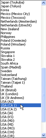
We examine a data set analyzed in Chapter 5 of Zuur et al. (2007) to illustrate how to fit ordinary linear regression models in R. The data here consist of the abundances of different marine invertebrate species collected at various sites in the North Sea off the coast of Holland. The stated goal in Zuur et al. (2007) is rather vague—to determine what abiotic factors affect the benthic fauna. Without there being a more specific research question we are straying into the realm of data dredging rather than true science, so we'll use the data for illustrative purposes only.
When R starts up you are presented with a console window in which you can enter commands. You can move back within a command line to correct mistakes by using the left and right arrow keys on the keyboard or with the mouse. The home and end keys can be used to move to the beginning and end of the current line. Previously issued commands can be recalled with the up arrow key.
The read.table function is used to read data into R from a text file. The data may reside in a file that is stored on your personal computer or at a location on the web. I first consider reading data from a local file that is stored in a folder on your personal computer.
There is a default location from which R will read and write files. To see what this is use the getwd function. R uses standard mathematical notation f(x,y,z) to specify functions and their arguments, so parentheses, ( ), are always required with functions although sometimes it is not necessary to specify any arguments. The getwd function has no arguments but still requires both parentheses.
Notice that R indicates a computer's folder hierarchy by using a forward slash, /, not the backward slash, \, of Windows. When you specify a pathname to R you must also use forward slashes. On Windows you also have the option of using double backslashes, \\, but never a single backslash. The single backslash is an escape character in R and is used for the internal formatting of text strings.
I've downloaded the data file from the class web site and stored it in a folder called "ecol 562" in the "Documents" folder of my computer. The file was saved as "RIKZ" but because it was saved as a text file it also has the extension ".txt" associated with it. Depending on how you've configured your computer the file extension may not be visible to you. Regardless, the correct name of the file is "RIKZ.txt".
The structure of the current file is particularly simple so we only need to specify two arguments to read.table.
To save the output of the read.table function we use the assignment operator, <- , to assign the output to an object in R. The arrow points in the direction of the assignment. We can also use the assignment arrow -> in which case the calculation should appear first, then ->, followed by the variable that is to get assigned the result of the calculation.
Note: The <- can be replaced with an = sign. The equal sign always assigns the result of the calculation on the right to the variable on the left of the equal sign. Thus it cannot be used to replace ->.
Method 1: Specify the folder as part of the name
We can read in the file RIKZ.txt with read.table as follows. I store the result in a variable I call rikz.
R treats any line that begins with a # symbol as a comment and ignores it. I will occasionally mix comments in with the code to annotate what's being done. They will be colored in green and start with a # symbol.
The sep argument of read.table can be used to tell R what the field delimiter is. By default read.table assumes the fields in the file are separated by spaces or tabs. Use sep=',' to indicate a comma-delimited file or sep='\t' to explicitly indicate a tab-delimited file. The current file is tab-delimited so the following will also successfully read in the file.
There are two other R functions for reading in data, read.csv and read.delim. These files assume the files are comma-delimited and tab-delimited, respectively, by calling read.table with the appropriate arguments for sep already filled in.
Method 2: First change the working directory
If all of our data sets are found in a specific folder it probably makes sense to make that directory the working directory and read the files in directly from there. The setwd function can be used to first change the folder that is identified as the working directory. It takes a single argument: the complete path to the folder, enclosed in quotes. Now when I use read.table I don't have to specify the folder that contains the file.
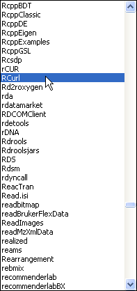
The read.table function can also be used to read in files from the web. For this the first argument of read.table is the URL of the file, where the entire URL is enclosed in quotes. This will work for files located on web sites whose URL begins with 'http://'. Unfortunately the Sakai site where the class files are stored is a secure site whose URL begins with "https://". Reading in public files from such sites is a two-step process in R that requires the use of the getURL function that is contained in the RCurl package. The RCurl package is not part of the standard installation of R so we'll first need to download it from the CRAN site and install it into our copy of R. This process needs to be done only once.
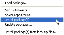
On Windows downloading and installing a new R package is a three-step process.
| (a) |
(b) |
(c) |
| Fig. 1 Windows OS: Installing an R package from the CRAN site on the web | ||
The desired package will be downloaded along with any additional packages it requires.
Choose Package Installer from the Packages & Data menu (Fig. 2a). In the window that appears (Fig. 2b) enter RCurl in the Package Search box and press the return key on the keyboard to search for the RCurl package. It should eventually appear in the Package column along with its version number. Click the Install Dependencies check box so that if the package depends on any other packages these will be downloaded also. Finally, highlight the desired package in the list (sometimes multiple packages appear) and click Install Selected to download the package to the R libraries folder.
(a) 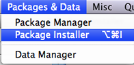 |
(b) 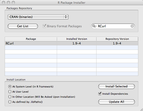 |
|
| Fig. 2 Mac OS X: Installing an R package from the CRAN site. | ||
If the package fails to turn up when searching for it, the CRAN mirror you're using doesn't have the appropriate version of the package for your installed version of R. In that case you can try changing the mirror by entering chooseCRANmirror() at the R command prompt in the console, choosing a different mirror site in the pop-up menu that appears, and repeating the above protocol to try to install the package again from the new site.
The package is now installed into your version of R but it hasn't been loaded into memory yet. That can be done with the library function.
The next step is to bring the text file into R from the web site with the getURL function from the RCurl package. This brings the contents of the file into R as a single long character string. In the command shown below I enclose the URL of the RIKZ data set from the Sakai web site in quotes and make it the first argument of getURL.
The above function call works on my Mac, but on Windows I get the following error message.
Error in function (type, msg, asError = TRUE) :I was able to fix this by adding two additional arguments to getURL, ssl.verifyhost=F and ssl.verifypeer=F.
Finally we need to convert the output from getURL into a usable format. The function textConnection will do this and the output from it can then be used as the first argument of read.table.
The object rikz that we've created in R is called a data frame. Data frames look like matrices but the elements of data frames can be mixtures of character and numeric data. More formally data frames are tightly coupled collections of variables that share many of the properties of matrices and of lists. They are the fundamental data structures for most of R's modeling functions.
The dim function is used to determine the dimensions of a data frame.
From the output we see that there are 45 rows and 89 columns. To display the contents of a data frame we can use the print function or just type the name of the data frame at the R prompt and press the Enter key. Because the rikz data set is so large, it makes more sense to just display a subset of the data set. For instance, the following displays the first four rows of rikz.
The notation 1:4 is shortcut for the numbers 1, 2, 3, 4. The bracket notation, [ ], is used to display the elements of a data frame. The value that precede the comma denotes the rows to be selected. The value that follows the comma denotes the columns. Because no numbers follow the comma in the above example, we obtain all 89 of the columns of the data frame.
In the above display we see that the variable names appear in the first row of the output and the row numbers appear in the first column. The display wraps to a new line when the window is full. The variable names that start with one or two capital letters followed by a number denote different marine invertebrate species that were collected in the various samples. The displayed values are the counts of individual organisms in the sample. A value of zero means the species was not observed in the current sample. In the last few columns are variables corresponding to the various abiotic measurements that were made. These will be the predictors in our regression model. In addition we see that there are variables denoting the sample number (Sample in column 1), as well as the week the measurement was made and the beach on which the measurement was taken.
To look at rows 1 through 4 but only columns 1 and 77 through 89 I enter the following. The c function is the catenate function. It concatenates in this case numbers that are not consecutive into a vector.
We can also select elements of a data frame using what's called list notation. In this notation we specify the name of the data frame followed by a $ sign followed by the name of the variable. For instance, rikz$NAP displays the values of the variable in the rikz data frame called NAP.
We can obtain the same output with the bracket notation by enclosing the name of the desired column in quotes.
When we examine the data more closely we see that we don't have a simple random sample of beach locations. If we tabulate the beach variable with the table function we see that there are five samples per beach.
So, at best we have a two-stage cluster sample in which a random sample of beaches was taken after which a random sample of five observations was taken on each beach. If we look at the variable week, things become even more complicated.
From the table of week versus beach we see that the different beaches were sampled in different weeks. Thus observations were not made at the same time but were obtained sequentially over the course of a month. This has the potential of introducing a temporal component to the data. It may turn out that observations are similar because they came from the same beach or because they were obtained during the same week, rather than because of any of the attributes that were measured. If the abiotic variables don't account for this spatial and temporal clustering it may be necessary to include it explicitly in the model.
There are also some issues with the abiotic variables. Below I look at the first 8 rows of the non-biological variables.
What we see is that values of some variables vary for each sample while some are the same for individual samples but vary only when we switch to another beach. Thus angle2, exposure, salinity, and temperature were apparently measured once on each beach but were not measured at individual sample locations. This raises the question of how these variables should be used in a regression model. If we use them as ordinary predictors we are forced to assume that the beach-level values accurately reflect what would have been measured at individual sample sites. The data set already gives us a reason to question this assumption. There are two reported angle measurements in the data set, angle1 measured at each sample location and angle2 measured for each beach. They don't look anything like each other.
The names function displays the names of the columns of a data frame. (The same output can also be obtained with the colnames function.)
The numbers at the edge of the display give us the position of the next displayed element in the vector of names. Using these numbers we see that the species data appear in columns 2 through 76. To calculate the species richness of a sample we need to count up the number species for which the recorded value is different from zero. A simple way to accomplish this is with the apply function. The apply function takes three arguments:
A nice description of the apply function as well as some of the other sophisticated R functions useful for manipulating entire matrices can be found on the UCLA stats web site.
http://www.ats.ucla.edu/stat/r/library/advanced_function_r.htm
Suppose we wanted to calculate the total abundance at each site. For that we would need to add up the counts for all the individual species. The following function call uses the apply function to do the job.
To obtain richness we need to determine if a species was present or absent at the site and then count the number of presences. We can determine if a species was present or absent by using the Boolean condition x > 0. This evaluates to TRUE if x is greater than zero, FALSE if x is 0 (or less). I try it out for the first site. In this case it yields a vector of length 75 consisting of individual TRUEs and FALSEs.
By default TRUE values have numeric value 1 and FALSE values have numeric value 0, so we can sum them to obtain the number of species that were present.
Now we're ready to calculate the richness of each of the individual sites. The following use of the apply function calculates the richness at each site and creates a new column in the data frame rikz with the name "richness".
If we examine the rikz data frame we see that a new column has been added.
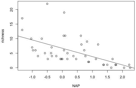
The variable NAP measures the height of a sample site relative to the mean tide level and is the first predictor considered by Zuur et al. (2007) in their regression model. The lm function of R fits ordinary regression models. The regression model itself is specified as a formula, in this case, richness ~ NAP. The data argument is used to specify the data frame that contains the variables that appear in the formula.
Entering the name of an R object at the prompt in the console window causes the object to be printed. With an lm object this yields a minimal amount of information about the model fit—just the call that was used and estimates of the parameters.
To get additional information we can use the summary function.
Residuals:
Min 1Q Median 3Q Max
-5.0675 -2.7607 -0.8029 1.3534 13.8723
Coefficients:
Estimate Std. Error t value Pr(>|t|)
(Intercept) 6.6857 0.6578 10.164 5.25e-13 ***
NAP -2.8669 0.6307 -4.545 4.42e-05 ***
---
Signif. codes: 0 ‘***’ 0.001 ‘**’ 0.01 ‘*’ 0.05 ‘.’ 0.1 ‘ ’ 1
Residual standard error: 4.16 on 43 degrees of freedom
Multiple R-squared: 0.3245, Adjusted R-squared: 0.3088
F-statistic: 20.66 on 1 and 43 DF, p-value: 4.418e-05
Two p-values appear in the output.
Notice that the two p-values are identical (when rounded to two decimals). That's because there is only one predictor in the model. In this special case the F-statistic (20.66) is equal to the square of the t-statistic (–4.545). We conclude that there is a statistically significant linear relationship between richness and NAP. Another useful quantity is R2, labeled "Multiple R-squared" in output. In words it tells us that 32.45% of the variability in the response has been explained by its linear relationship with NAP.
Scatter plots are produced with the plot function. We can use formula notation in the plot function as follows.
The plot function is a high-level graphics command and will cause the contents of the active graphics window to be replaced with the current graph. Other graphics commands can then be used to add additional features to the current graph. The abline function can be used to add a regression line to the current graph. When there is only one predictor abline needs only the lm object in order to draw the line (Fig. 3).
 |
|
| Fig. 3 Regression model superimposed on a scatter plot of the data. | |
I next consider adding the structural variable, week, to the regression model. Even though this variable has numeric values, it is in fact a categorical variable. The values just serve to label the categories. Because the labels also serve to order the categories it might be tempting to treat it as continuous. This would not be wrong but when we treat it as categorical we'll be able to see if linearity is a good assumption. To make R treat week as categorical I use the factor function of R when fitting the model. The factor function automatically creates a set of indicator variables using the lowest numeric value to define the baseline level. For the variable week R generates the following regressors.
 ,
,  ,
, 
We can verify that this is the case by using the levels and contrasts functions of R on the factor variable.
The output from levels tells us that R sees four categories that it is labeling (notice the quotes around the values) 1, 2, 3, and 4. The contrasts function shows the coding of the three dummy variables (the three columns in the displayed output) for each of the four categories of week (the four rows in the output). Observe that the reference level, week = 1, has a value of zero in each of the three columns.
First I fit the additive model.
![]()
This is a model in which we have a different regression line (richness versus NAP) for every week. The lines are parallel but are allowed to have different intercepts. (See lecture 2.)
Next I fit the interaction model. This allows the lines to have different slopes and different intercepts in each week. Interactions in R are denoted with a colon, NAP:factor(week).
Alternatively we can use R's shortcut * notation to fit this model.
The asterisk between the terms causes R to generate the individual terms plus the interaction term. The interaction model written in terms of the dummy variables defined above is the following. (See lecture 2.)
![]()
This is also a model in which we have a different regression line (richness versus NAP) in every week. It differs from the additive model in that the lines are now allowed to have both different slopes and different intercepts.
The three models we've fit so far are nested. We can reduce the interaction model (mod3) to the additive model (mod2) by dropping the interaction terms. The can be expressed formally in the form of the following hypothesis test.
The anova function of R carries out this test. When anova is given a single model it carries out a sequence of partial F-tests starting with the individual additive terms and culminating with the interactions. These are sequential tests so that in each row of the output table, the term that appears in that row has been added to a model that already contained all the terms listed above it in the table. The anova function adheres to the principle of marginality so that a model with an interaction term must also contain the main effect terms that comprise the interaction. A good way to read the table produced by the anova function is from the bottom up.
Response: richness
Df Sum Sq Mean Sq F value Pr(>F)
NAP 1 357.53 357.53 59.9605 2.967e-09 ***
factor(week) 3 387.11 129.04 21.6406 2.896e-08 ***
NAP:factor(week) 3 136.38 45.46 7.6241 0.0004323 ***
Residuals 37 220.62 5.96
---
Signif. codes: 0 ‘***’ 0.001 ‘**’ 0.01 ‘*’ 0.05 ‘.’ 0.1 ‘ ’ 1
The row labeled NAP:factor(week) tests whether we need to add an interaction term to the additive model. Because the p-value of the test is small (p < .05), we reject the null hypothesis of no interaction and conclude the interaction of NAP and categorical week is statistically significant.
If we use the summary function on the fitted interaction model, mod3, we are shown the individual coefficient estimates for the different dummy regressors and the individual statistical tests for these coefficients. Because week 1 is the reference group, the tests involving the dummy regressors are tests of whether the slope or intercept in a given week is different from what it was in week 1. For example, the last line of the table tells us that the slope in week 4 is significantly different from what it was in week 1. From the reported point estimates we see that the slope in week 1 was –1.9 and the slope in week 4 is 7 less than this, or –8.9.
Residuals:
Min 1Q Median 3Q Max
-6.3022 -0.9442 -0.2946 0.3383 7.7103
Coefficients:
Estimate Std. Error t value Pr(>|t|)
(Intercept) 11.40561 0.77730 14.673 < 2e-16 ***
NAP -1.90016 0.87000 -2.184 0.035369 *
factor(week)2 -8.04029 1.05519 -7.620 4.30e-09 ***
factor(week)3 -6.37154 1.03168 -6.176 3.63e-07 ***
factor(week)4 1.37721 1.60036 0.861 0.395020
NAP:factor(week)2 0.42558 1.12008 0.380 0.706152
NAP:factor(week)3 -0.01344 1.04246 -0.013 0.989782
NAP:factor(week)4 -7.00002 1.68721 -4.149 0.000188 ***
---
Signif. codes: 0 ‘***’ 0.001 ‘**’ 0.01 ‘*’ 0.05 ‘.’ 0.1 ‘ ’ 1
Residual standard error: 2.442 on 37 degrees of freedom
Multiple R-squared: 0.7997, Adjusted R-squared: 0.7618
F-statistic: 21.11 on 7 and 37 DF, p-value: 3.935e-11
We can extract just the parameter estimates from the model with the coef function.
Using the dummy variable definitions given above we can calculate the intercept and slope of the lines in each of the four weeks. (See lecture 2.)
![]()
| Table 1 Intercepts and slopes for the regression lines in different weeks |
week |
intercept |
estimate of intercept |
slope |
estimate of slope |
1 |
β0 | coef(mod1)[1] | β1 | coef(mod1)[2] |
2 |
β0 + β2 | coef(mod1)[1] + coef(mod1)[3] | β1 + β5 | coef(mod1)[2] + coef(mod1)[6] |
3 |
β0 + β3 | coef(mod1)[1] + coef(mod1)[4] | β1 + β6 | coef(mod1)[2] + coef(mod1)[7] |
4 |
β0 + β4 | coef(mod1)[1] + coef(mod1)[5] | β1 + β7 | coef(mod1)[2] + coef(mod1)[8] |
Using this information we can plot the individual lines estimated by the model. I do this two ways: first using base graphics of R and secondly using the lattice package.
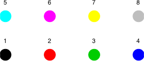
Using base graphics I plot all the data in single scatter plot using different colors and plotting symbols to represent the data from different weeks. This is accomplished by including the col and pch arguments in the plot function and choosing values from those shown in Fig. 4 below. R has 25 built-in plotting symbols and over 600 named colors as well as 8 colors that can be specified with the numbers 1 through 8. To see a full list of colors go to http://research.stowers-institute.org/efg/R/Color/Chart/index.htm.
 |
 |
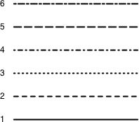 |
| Fig. 4 Plotting characters (pch), numeric color codes (col), and line types (lty) in R | ||
Because the variable week is coded 1 through 4, I can use the value of week as the argument to col to select one of the first four numbered colors, col = week. I elect to use the filled plotting symbols that start with 15. These can be obtained by adding 14 to the value of week, pch = 14 + week.
If week was a factor (e.g., if it was originally a character variable and was then converted to a factor by R when it was read in by the read.table function), the same effect could be obtained with the as.numeric function.
To add the regression lines to the plot I use the abline function. I give the intercept as the first argument and the slope as the second argument to abline. The values are determined from the formulas given in Table 1. I specify the appropriate color with col= and make the line dashed by specifying lty=2.
Finally I add a legend to distinguish the lines and plotting symbols.
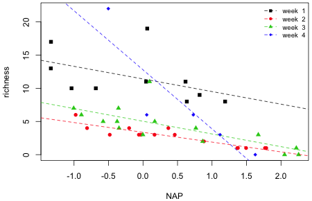
The final graph is shown in Fig. 5.
 |
|
| Fig. 5 Interaction model superimposed on a scatter plot of the data. | |
From the graph it appears that it is week 4 that is driving the interaction. The lines in the other three weeks are roughly parallel. It also appears that there is a single site with a very large richness value that has been highly influential on the fit. Given that only five sites are being used to estimate the slope and intercept in week 4, the regression line for week 4 does not appear to be very reliable.
The lattice package provides a second way to create graphs in R. (A third way is with the ggplot2 package.) Although lattice can be used to produce any graph that base graphics can produce, the primary use of the lattice package is to generate panel graphs (trellis graphics) in which we plot a relationship between variables conditional on the value of some other variable. In the present example we will use week as the conditioning variable.
The lattice package is part of the standard installation of R so we don't need to download it from the web. We do first need to load it into memory though.
The primary plotting function in lattice is the xyplot function. It supports the formula notation we used in the plot function. To indicate that we want a separate plot for each week we write the formula as follows: richness~NAP|week.
The labeling of the panels is less than ideal in Fig. 6a. Because week is a numeric variable lattice has used a thermomenter-like display to indicate its relative value. To get the actual values of each week to display in the panel we need to convert week to a factor.
Finally we can get slightly nicer labels by generating our own text for them in the call to the factor function. I include the levels argument to indicate what the levels are and the labels argument to associate the desired labels with those levels.
Fig 6b shows the result.
(a) 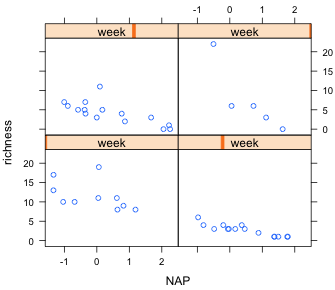 |
(b) 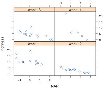 |
|
| Fig. 6 A panel graph in which the grouping variable week is treated (a) as a continuous variable, and (b) as a factor. | ||
The arrangement of the panels is determined by size of the graphics window. The arrangement can be specified explicitly with the layout argument. For example, to have the panels arranged in one column and four rows we would add the argument layout=c(1,4) to the xyplot call.
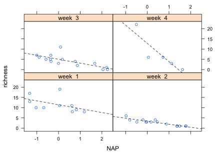
What's shown in the individual panels is determined by a panel function. The default panel function just the displays a scatter plot of the data. To add a regression line we need to write our own panel function. This is done by specifying the panel argument of the xyplot function followed by our function definition. A panel function that produces a scatter plot of the points and adds dashed regression lines is shown below. Because the function has more than one line we need to enclose the lines in a pair of curly brackets, { }.
panel.xyplot and panel.lmline are special functions that are used only when defining a panel function. Here's the full call to xyplot with the user-specified panel function.
Fig. 7 shows the result. One of the nice features of the lattice package is that the graph in each panel is drawn to the same scale (this can be overridden) so that the points and lines in the different panels are directly comparable.
 |
|
| Fig. 7 Graph of the interaction model using the lattice package | |
In Windows the history function can be used to display recent lines of code. For instance,
will display in a separate window the last 100 lines of code that you've entered in the R command console. The contents of this window can then be saved or you can copy out selected lines of code from this window.
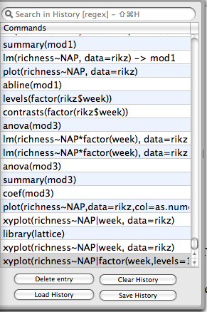
This method doesn't work in Mac OSX. Instead you should click the icon at the top of the screen that is indicated in Fig. 8. This opens a history window next to the console window which has buttons that allow you to save the contents of the history window to a file. The saved file is given the extension .Rhistory, but it is really a text file and can be opened and edited with a text editor such as TextEdit or a word processor.
 |
 |
| Fig. 8 Saving the history of R commands in Mac OSX |
When you shut down R you will be prompted to save the current R workspace. The R workspace consists of all the objects you created in the current R session (and whatever objects were saved from previous sessions). Generally speaking you will not want to save the workspace. Instead when you open R the next time, use the saved history of commands (after editing out the mistakes you made) to regenerate those objects that you need. That way you start with a clean slate each time.
Zuur, Alain F., Elena N. Ieno, and Graham M. Smith. 2007. Analysing Ecological Data. Springer, New York. UNC e-book
| Jack Weiss Phone: (919) 962-5930 E-Mail: jack_weiss@unc.edu Address: Curriculum of the Environment and Ecology, Box 3275, University of North Carolina, Chapel Hill, 27599 Copyright © 2012 Last Revised--Jan 15, 2012 URL: https://sakai.unc.edu/access/content/group/2842013b-58f5-4453-aa8d-3e01bacbfc3d/public/Ecol562_Spring2012/docs/lectures/lecture3.htm |