Lecture 13—Wednesday, February 8, 2012

Topics

• Deviance
  • The deviance as a goodness of fit statistic
  • Analysis of deviance
• Residuals for generalized linear models
  • Deviance residuals
  • Pearson residuals
• Binomial distribution
• Logistic regression
• Interpreting regression equations with different link functions
  • Identity link
  • Log link
  • Logit link
• Cited references

Deviance

The deviance as a goodness of fit statistic

Historically a quantity called the deviance has played a large role in assessing the fit of generalized linear models. The deviance derives from the usual likelihood ratio statistic as we now illustrate. Suppose we have two nested models with estimated parameter sets and and corresponding likelihoods and . If is a special case of then we can compare the models using a likelihood ratio test.

Recall that LR has an asymptotic chi-squared distribution with degrees of freedom equal to the difference in the number of parameters estimated in the two models. Alternatively, the degrees of freedom is the number of parameters that are fixed to have a specific value in one model but are freely estimated in the other model.

A saturated model is one in which one parameter is estimated for each observation. Suppose the model with likelihood is the saturated model and is the likelihood of some model of interest, call it model M. In the special case where model M is being compared to the saturated model, the likelihood ratio statistic for this comparison is called the deviance. Technically a distinction is made between the residual deviance, D_M , and the scaled deviance, the residual deviance divided by the scale parameter.

The scale parameter is a term recognizable in the log-likelihood when it is written in its exponential form. For the Poisson and binomial distributions, the two probability models for which the deviance can be legitimately used as a goodness of fit statistic, this distinction between residual deviance and scaled deviance is unimportant because the scale parameter φ = 1, so the two are the same.

In the saturated model n parameters are estimated, one for each of the n observations. In model M there are p < n parameters that are estimated. This means that n – p of the parameters that were estimated in the saturated model are set to zero in Model M. Because the scaled deviance is a likelihood ratio statistic it follows that

Thus the deviance has the form of a goodness of fit statistic. Large values of the deviance, relative to its degrees of freedom, indicate a significant lack of fit. As was noted above there are only two kinds of generalized linear models for which the deviance is an appropriate goodness of fit statistic: Poisson regression and logistic regression with grouped binary data (which we'll consider in lecture 14). The deviance statistic should not be used as a goodness of fit statistic for logistic regression with a binary response.

The mean of a chi-squared distribution is equal to its degrees of freedom, i.e., . Thus if a model provides a good fit to the data and the chi-squared distribution of the deviance holds, we expect the scaled deviance of the model to be close to its mean value n – p, i.e., . For Poisson and binomial probability models, φ = 1. Thus for these models we expect or equivalently . So a quick test of the adequacy of a Poisson or binomial model is to divide the residual deviance by its degrees of freedom and see if the result is close to one. If the ratio is much larger than one we call the data overdispersed. If it is much smaller than one we call the data underdispersed. (Note: The use of these terms should be restricted to Poisson and binomial distributions.)

Unfortunately the accuracy of this test is somewhat dubious with small data sets. In order for the chi-squared distribution of the deviance to hold, the expected Poisson or binomial counts, i.e., the fitted values predicted by the model, should be large. A general rule is that they should exceed 5, although when there are many categories Agresti (2002) notes that an expected cell frequency as small as 1 is okay as long as no more than 20% of the expected counts are less than 5.

To illustrate the use of the deviance for checking model fit we revisit a Poisson regression model that was fit in lecture 11.

To fit the saturated model we create a variable that has a different value for each observation, convert it to a factor, and then use it as a predictor in a Poisson regression model.

So in the saturated model we have 280 parameters, one for each observation. To compare our model to the saturated model we can use a likelihood ratio test.

The degrees of freedom of the likelihood ratio statistic is just the difference in number of parameters fit in the two models.

This likelihood ratio statistic and its degrees of freedom are reported as part of the summary output from the model and labeled the residual deviance.

Deviance Residuals:
     Min        1Q    Median        3Q       Max 
-12.0267   -2.6401   -1.5599    0.1912   20.9158 

Coefficients:
                   Estimate Std. Error z value Pr(>|z|)   
(Intercept)      -0.0349466  0.0911488  -0.383    0.701   
CORAL_COVE        0.0332184  0.0018308  18.144   <2e-16 ***
WSSTA             0.3056099  0.0162077  18.856   <2e-16 ***
I(WSSTA^2)       -0.0270397  0.0007945 -34.032   <2e-16 ***
CORAL_COVE:WSSTA  0.0038035  0.0002341  16.246   <2e-16 ***
---
Signif. codes:  0 ‘***’ 0.001 ‘**’ 0.01 ‘*’ 0.05 ‘.’ 0.1 ‘ ’ 1

(Dispersion parameter for poisson family taken to be 1)

    Null deviance: 11827.0  on 279  degrees of freedom
Residual deviance:  4912.3  on 275  degrees of freedom
AIC: 5527.6

Number of Fisher Scoring iterations: 7

To carry out the deviance goodness of fit test we compare the deviance to the critical value of a chi-squared distribution with 275 degrees of freedom. The p-value of the residual deviance is

Because the p-value is very small, we should reject the null hypothesis. Before we conclude that we have a significant lack of fit, we should verify that our data meet the minimum sample size criteria. We calculate the expected counts and determine the fraction of them that are less than 5.

So 55% of the expected cell counts are less than five. This is far greater than 20% suggesting that we should not take the deviance test seriously here.

Analysis of deviance

The likelihood ratio test is often written with a negative sign.

Written this way L₁ is the larger of the two models (it has more estimated parameters) and L₀ is the simpler model in which some of those parameters have been assigned specific values (such as zero). Written this way and letting L_S denote the likelihood of the saturated model, the scaled deviance can be written as follows.

Now suppose we wish to compare two nested models with likelihoods L₁ and L₂ in which L₂ is the "larger" (more estimated parameters) of the two likelihoods. The likelihood ratio statistic for comparing these two models, written in the alternate format given above, is the following.

where D₁ and D₂ are the deviances of models 1 and 2, respectively. Thus to carry out a likelihood ratio test to compare two models we can equivalently just compute the difference of their scaled deviances.

Because of the parallel to analysis of variance (ANOVA) in ordinary linear models, carrying out an LR test using the scaled deviances of the models is often called analysis of deviance. This is what is reported by the anova function in R. The column labeled "Deviance" really represents the change in deviance between two adjacent models in the table. These are also likelihood ratio statistics.

Model: poisson, link: log

Response: PREV_1

Terms added sequentially (first to last)

                 Df Deviance Resid. Df Resid. Dev  Pr(>Chi)   
NULL                               279    11827.0             
CORAL_COVE        1   4617.5       278     7209.5 < 2.2e-16 ***
WSSTA             1     51.4       277     7158.0 7.371e-13 ***
I(WSSTA^2)        1   1967.7       276     5190.4 < 2.2e-16 ***
CORAL_COVE:WSSTA  1    278.1       275     4912.3 < 2.2e-16 ***
---
Signif. codes:  0 ‘***’ 0.001 ‘**’ 0.01 ‘*’ 0.05 ‘.’ 0.1 ‘ ’ 1

Residuals for generalized linear models

In the ordinary normal-based multiple regression model, we write

where ε_i is referred to as the error. When we obtain estimates for the parameters we write the fitted model as

so that is an estimate of the errors, ε_i. The e_i are called residuals, or more properly, the raw residuals (also called the response residuals) of the model. For generalized linear models the raw residuals are seldom useful. Instead two other kinds of residuals, deviance residuals and Pearson residuals, are used.

Deviance residuals

The deviance is twice the difference in log-likelihoods between the current model and a saturated model.

Because the likelihood is a product of probabilities or densities, each log-likelihood is a sum of a probability or density for each observation. If we group the corresponding log-likelihood terms from both the model and the saturated model by observation, we get that observation's contribution to the deviance which we denote by . Because of the factor of two that multiplies the difference in logs, each of these contributions is squared, . The deviance residual is defined as follows.

Here sign denotes the sign function which is defined as follows.

Because under ideal conditions the deviance can be used as a measure of lack of fit, the deviance residual measures the i^th observation's contribution to model lack of fit.

Pearson residuals

The Pearson residual is a standardized raw residual. The raw residual is divided by an estimate of the standard error of the prediction.

This estimate will vary depending on the probability distribution chosen for the response. The Pearson residual is that observation's contribution to the Pearson goodness of fit statistic.

Binomial distribution

A binomial random variable is discrete. It records the number of successes out of n trials. The classic illustration of the binomial distribution is an experiment in which we record the number of heads obtained when a coin is flipped n times. A binomial random variable is bounded on both sides—below by 0, above by n. This distinguishes it from a Poisson random variable which is bounded below by zero but is unbounded above.

An experiment is called a binomial experiment if four assumptions are met.

1. Each trial is a Bernoulli trial, meaning that only one of two outcomes can occur. The outcomes are generally referred to "success" and "failure".
2. The number of trials is fixed ahead of time and is denoted by n.
3. The probability p of a success is the same on each Bernoulli trial.
4. The individual Bernoulli trials are independent.

The binomial is a two-parameter distribution with parameters n and p. We write. The mean and variance are

Observe from this last expression that the variance is a function of the mean, i.e., . If you plot the variance of the binomial distribution against the mean you obtain a parabola opening downward with a maximum at corresponding to p = 0.5. When n = 1 the binomial distribution is sometimes called the Bernoulli distribution and the data are referred to as binary data. To contrast this situation from the binomial distribution proper, we will refer to data arising from a binomial distribution with n > 1 as grouped binary data.

Examples of binomial data

• A seed germination experiment (binomial data proper). An experiment is carried out in which 100 seeds are planted in a pot and the number of seeds that germinate is recorded. This is done repeatedly for pots subjected to various light regimes, burial depths, etc. Clearly the first two assumptions of the binomial model hold here: the outcome on individual trials is dichotomous (seed germinates or seed did not germinate) and the number of trials was fixed ahead of time at 100. The remaining two assumptions (constant p and independence) would need to be verified.
• The spatial distribution of endangered species (binary data). We record the presence-absence of the species in a habitat (using perhaps a set of randomly located quadrats). We then try to relate the observed species distribution to characteristics of the habitat. The presence or absence of the species in a given quadrat is a realization of a binomial random variable with n = 1.

R binomial functions are denoted: dbinom, pbinom, qbinom, rbinom. In R the parameters n and p are specified with the argument names size and prob respectively. There is no special function for binary data in R. Just use the binomial function and set size = 1 (n = 1).

Logistic Regression

Logistic regression is the preferred method of analysis for situations in which the response has a binomial distribution. Logistic regression is a generalized linear model in which

1. the random component is the binomial (Bernoulli) distribution,
2. the linear predictor is , and
3. the link function is , also called the logit.

When the binomial distribution is put in its standard exponential form the parameter p only occurs as part of the logit function . For this reason the logit function is called the canonical link in logistic regression. The logit turns out to be an excellent choice as a link function. One of the problems with using the identity link for proportions is that although proportions are required to lie in the interval [0, 1], an identity link can yield predictions outside this interval. The logit function restricts p to the unit interval as we now demonstrate. Setting the logit link equal to the linear predictor and solving for p yields the following.

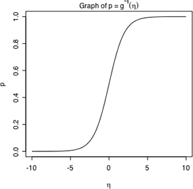
Fig. 1  Inverse of the logit link

The expression that inverts the logit link is called the logistic function and is shown in Fig. 1. Observe the following.

• Since η is the linear predictor there are no restrictions on its values and it in principle can range from –∞ to ∞.
• The exponential function is always positive. Therefore the expression is also always positive.
• Because is always positive it follows that . Hence .
• approaches 0 as .
• approaches 1 as .
• Therefore the logistic function maps the linear predictor η nonlinearly into the interval (0, 1).

Other suitable link functions for binomial data are the probit, , and the complementary log-log link, , but the logit is certainly the most popular choice. The reason the logit is the preferred link function for binomial data is that it is interpretable. We examine this interpretation next.

Interpreting regression equations with different link functions

As a background for understanding how to interpret regression coefficients in models with a logit link, we review the interpretation of regression coefficients in other kinds of regression models.

Identity link

When is the identity function, as is typically the case in ordinary linear regression, then

.

If we increase x₁ by one unit, then we have

So β₁ is interpreted as the amount that the mean is increased when x₁ is increased by one unit.

Log link

When is the log function, as in Poisson or negative binomial regression, then

If we increase x₁ by one unit, then we have

So β₁ is the amount that the log mean is increased when x₁ is increased by one unit. Converting to the original scale of the mean we have the following.

So we can interpret β₁ in terms of , which is the amount the mean is multiplied by when x₁ is increased by one unit.

Logit link

The argument just given in which we invert the identity and log links does not work for the logit link. The regression coefficients do not have simple interpretations on the scale of p, the probability of success. On the other hand the regression coefficients in logistic regression do have a simple interpretation in terms of the odds. Probability theory had its origin in the study of gambling. Gamblers typically speak in terms of the "odds for" or "odds against" events occurring, rather than in terms of probabilities, but the two notions are equivalent. Any statement made using odds can also be expressed in terms of probability.

As an example, suppose it is stated that the odds in favor of an event Y = 1 occurring are 3 to 1. This can be interpreted as follows.

Thus if the odds for an event are 3:1, then the event has a probability of occurring.

Notice that it is odds, rather than probability, that is the argument of the logarithm function in the logit link. Thus the logit function is also called the log odds function. When the logit is viewed as a log odds, this immediately provides us with an interpretation for the regression parameter β₁ in the logistic regression model. Switching to the log odds notation we have the following.

Solving for β₁ yields the following.

where the notation OR denotes the odds ratio, the ratio of two odds. The specific odds ratio shown here measures the effect of increasing x₁ by 1 on the odds that Y = 1.

Just as is the case with ordinary regression, Poisson regression, and negative binomial regression, we can use the sign of the regression coefficient in logistic regression to infer the effect a predictor has on the response. If β₁ is the regression coefficient of x₁in the logistic regression model we have the following.

• If β₁ > 0 then > 1 and the odds of Y = 1 occurring go up when x₁ increases.
• If β₁ < 0 then < 1 and the odds of Y =1 occurring go down when x₁ increases.

Cited references

• Agresti, Alan. 2002. Categorical Data Analysis. Wiley: New York.

Course Home Page