Lecture 12—Monday, February 6, 2012

Topics

• Negative binomial distribution
  • Basic properties and characteristics
  • Graphs of different negative binomial distributions
  • Theoretical motivations for the negative binomial distribution
• Generalized linear models
  • The limitations of ordinary regression models
  • The defining characteristics of generalized linear models
  • Ordinary regression models are generalized linear models
  • Link functions
• Cited references

Negative binomial distribution

In lecture 11 we gave some basic information about the negative binomial distribution and used it as the probability model for the response in a regression problem. Here we restate the basic properties of this distribution, give some examples of its flexibility, and provide some motivation for why the negative binomial distribution is particularly suitable as a probability model for count data in ecology.

Basic properties and characteristics

A negative binomial (NB) random variable is discrete. Like the Poisson distribution it is bounded below by 0 but is theoretically unbounded above. A typical use of the negative binomial distribution is as a model for count data. An example would be in describing the number of cases of Lyme disease in a North Carolina county in a year.

There are two distinct parameterizations of the negative binomial. One parameterization appears in most introductory probability texts and the second appears in most ecology texts. In the ecological parameterization there are two parameters: μ and θ. μ is the mean and θ is the dispersion parameter. θ is also called the size (in R) or the scale parameter. θ is defined differently in different statistical packages. For example in SAS the dispersion parameter for the negative binomial is the reciprocal of the one reported by R.

The mean of the negative binomial distribution is μ. The variance of the negative binomial distribution is . Thus the variance is a quadratic function of the mean. Contrast this with the variance-mean relationship for the Poisson where the variance is equal to the mean. Using the R parameterization, if we let the dispersion parameter go to infinity the random variable that results is a Poisson random variable with parameter μ, i.e., if then . The R negative binomial probability functions are dnbinom, pnbinom, qnbinom, rnbinom.

Graphs of different negative binomial distributions

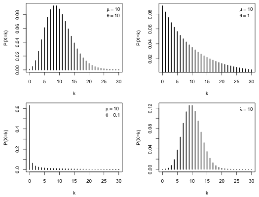
To appreciate the flexibility of the negative binomial distribution and to understand the role θ plays we graph a number of negative binomial distributions that have the same mean but have different values of θ. In the example below I fix the mean at 10 and set θ equal to 10, 1, and 0.1. For comparison I also show a Poisson distribution with a mean of 10. The plots are arranged in a 2 × 2 grid using the mfrow argument of par.

Fig. 1  Three negative binomial distributions with μ = 10 but with θ = 10, 1, and 0.1. A Poisson distribution with λ = 10 is included for comparison.

As the plots reveal varying θ can have a dramatic effect on the shape of the distribution. As θ gets larger the negative binomial distribution more closely approaches a Poisson distribution with the same mean. One thing that is perhaps not apparent from the graphs is how much more probable extreme values are under a negative binomial distribution. The code below calculates the probability of observing a count of 30 under the three negative binomial models in Fig. 1 and also under the Poisson distribution. Notice that for all three negative binomial distributions observing a count of 30 is at least 1000 times more likely than it is for a Poisson distribution with the same mean.

Obtaining both very large and very small counts is quite likely with a negative binomial distribution. With a Poisson distribution such a combination is essentially impossible.

Theoretical motivations for the negative binomial distribution

Boswell and Patil (1970) list 12 distinct ways in which a negative binomial distribution can arise in practice. Of these only three appear to have much relevance to environmental science. Each is a consequence of violating a specific assumption of the Poisson distribution. The assumptions of the Poisson distribution were given in lecture 10 and are repeated below.

1. Homogeneity assumption. Events occur at a constant rate λ such that on average for any length of time t we would expect to see λt events. If the events are occurring over space then for an area of size A we would expect to see λA events.
2. Independence assumption. For any two non-overlapping intervals (or areas) the numbers of observed events are independent.
3. If the interval is very small, then the probability of observing two or more events in that interval is essentially zero.

Here are three ways the negative binomial distribution can arise from violations of a Poisson distribution.

1. Nonhomogeneous Poisson process. If X is Poisson but λ is not constant and instead varies from place to place, or from time to time, then it is said that we have a nonhomogeneous Poisson process. If we're willing to make a specific assumption about how λ varies we are led directly to a negative binomial distribution. More specifically, if λ has a gamma distribution (a very flexible distribution), and X, conditional on the value of λ, has a Poisson distribution, then X, unconditionally, will have a negative binomial distribution. In this scenario the gamma distribution is called a mixing distribution.

   It turns out there are two ways the conditioning can be done and they yield different mean-variance relationships. One method yields a linear mean-variance relationship, , where k is constant. Notice that the Poisson is a special case of this with k = 1. This is called the NB1 model in the econometrics literature. The second method yields the mean-variance relationship given above, . This is sometimes called the NB2 model.

2. Independence. If we relax the independence assumption of the Poisson model in a special way so that the occurrence of one event makes the occurrence of the next event more likely, we get a negative binomial distribution. The special way to relax independence is called a Polya-Eggenberger urn model. This is one of the many so-called Polya urn models that exist in the literature. The description of this urn model is as follows.
   • Suppose we have an urn with N balls in it of which a fraction p are red and the remaining fraction 1 – p are black.
   • At each trial we draw one ball from the urn, observe its color, and return it to the urn along with θ × N balls of the same color (where usually we take 0 < θ < 1 although this is not required). By adding more balls of the same color we make the occurrence of the same event at the next trial more likely.
   • Let X_r= number of red balls in the urn after r trials of this sort. It is not hard to write down the formula for but it is rather involved, particularly the simplification that is required to proceed further, so we'll skip it.
   • It can be shown that if we take the limit of this expression in a certain way, i.e., while , then the limiting distribution is negative binomial.

   It's hard to know how useful this result is in practice. What is important is that the Polya-Eggenberger scheme clearly violates the independent increments hypothesis that was one of the three basic assumptions of the Poisson model. Thus we see that if either one of the major assumptions of the Poisson model, homogeneity or independence, is violated we can be led, under certain circumstances, to a negative binomial model.

3. Generalized Poisson model. Suppose that events are actually clustered and that the clusters have a Poisson distribution. Suppose within each cluster the number of observed events follows a logarithmic distribution (also called a log series distribution). This is a particular long-tailed distribution that has been used to model species abundances (Dewdney 2000). Now suppose we lay down a grid, not realizing that there are clusters present, and just count up the events we see in the cells of our grid. The distribution of the counts that results is negative binomial.

It is easy to imagine each of these three mechanisms occurring in practice.

• Suppose seeds are randomly distributed in an environment (governed by a Poisson model) and that each seed germinates and gives rise to a number of stems via vegetative reproduction, the number of stems governed largely by how long the plant has been present in the environment. The generalized Poisson model suggests that this might yield a negative binomial distribution for the number of plants present.
• Suppose the seeds of a plant species are heterogeneous in their propensity to germinate. This would imply a nonconstant λ in a Poisson model yielding a nonhomogeneous Poisson process. This may lead to a negative binomial distribution of counts of the number of adults we see in a habitat.
• In the case of a contagious disease where initial inoculates are distributed randomly according to a Poisson process, the Polya-Eggenberger urn model suggests we might end up with a distribution that is negative binomial.

A further application of the negative binomial distribution is with zero-inflated count data (meaning that we see more zeros than a fitted Poisson model can predict). The negative binomial distribution can often be successfully fit to zero-inflated data.

The negative binomial distribution is useful as a model for count data whenever we suspect heterogeneous rates of occurrence, lack of independence, clustering, or zero inflation.

Generalized linear models

Generalized linear models are regression models that include the normal regression model as a special case. They extend linear regression to probability distributions that are members of the exponential family of distributions. These include the normal, Poisson, binomial, and gamma distributions, among others. The negative binomial distribution is technically not a member of this group but it is possible to extend the methodology to include it. Generalized linear models were developed to fix the various problems we've already encountered with normal regression models.

The limitations of ordinary regression models

1. Response variables of interest in ecology are often not normally distributed nor do they tend to exhibit constant variance. While transformations can sometimes "fix" one or both of these problems, transformations introduce their own baggage and make the resulting model difficult to interpret. There's also no guarantee that a suitable transformation will be found.
2. Response variables may have a restricted range. For instance count data are required to be non-negative and proportions are required to lie between zero and one. The normal distribution does not have such a range restriction and hence may not be an appropriate probability model for such data.
3. It is often observed in ecological data that the variance is a function of the mean. This is especially true of restricted range data when values are near the boundary of their natural range. Limited range data near a boundary will necessarily exhibit a skewed distribution because of truncation at the boundary. This in turn limits the amount of variability they can display, at least in one direction.
4. The use of an identity link can cause problems. Because predictors do not have the same range restrictions as does the response variable, the systematic component can yield predicted values of the mean outside the legal range of the data.

The defining characteristics of generalized linear models

Generalized linear models (GLIMs) were designed to overcome the limitations described above. Proposed in the 1970s by McCullagh and Nelder (McCullagh and Nelder, 1989), GLIMs serve to unify a number of disparate modeling protocols under a single umbrella. While some revisionist statisticians think the significance of the GLIM paradigm is overstated (Lindsey 2004), I think it is fair to say that generalized linear models did for statistical modeling what plate tectonics did for geology. GLIMs provided a unifying vision to statistical modeling and brought a degree of order to what was otherwise a set of rather chaotic and seemingly arbitrary collection of procedures.

Formally a generalized linear model consists of the following three components.

1. Random component. The response variables Y₁, Y₂, … , Y_n are assumed to be independent and drawn from a member of the exponential family of distributions. The exponential family includes many of the standard probability distributions including the Poisson, normal, binomial, gamma, and inverse Gaussian distributions. (The negative binomial can be forced into the exponential family if the overdispersion parameter is treated as a constant.) Thus the normality and constant variance assumptions are relaxed for GLIMs.
2. Systematic component. The p covariates are combined to form a linear predictor. The linear predictor is typically denoted by the Greek letter η (eta). . This assumption is identical for both ordinary regression models and GLIMs.
3. Link function. The systematic component and random component are linked together via a link function g. For GLIMs the link function g can be selected from a large class of functions, although there are certain natural choices called canonical links. The only restriction on g is that it be differentiable and monotonic. Thus for a GLIM we write the regression model as follows.

Because we require g to be monotonic, it follows that g is invertible. Thus we can also write this last expression in terms of the inverse link function, .

Written this way we can see that GLIMs have the potential of solving the range restriction problem described above. Because the linear predictor is connected to the mean through , a judicious choice of link function can constrain the predictions to map onto a desired range. The so-called canonical link functions for the normal, Poisson, binomial, and gamma distributions are respectively the identity, log, logit, and reciprocal links. In most software packages a log link is used for the negative binomial distribution.

Ordinary regression models are generalized linear models

To see that normal regression models are also generalized linear models, we identify the random component, the systematic component, and the link function.

1. Random component: The response variables Y₁, Y₂, … , Y_n are assumed to be independent and normally distributed. More formally we assume . Observe that the mean is allowed to vary for each Y_i but that the variance does not.
2. Systematic component: The p covariates are combined to form a linear predictor. The linear predictor is represented by the Greek letter η (eta).
3. Link function: The systematic component and random component are linked together via a link function g(μ) = η. For ordinary regression models the function g is taken to be the identity link, g(μ) = μ, so that we assume μ = η . Using E to denote expectation, the operation of taking the mean, we can write this assumption as follows.

Link functions

Table 1 lists the probability distributions typically used as the random component in generalized linear models along with their canonical and usual link functions. When a probability distribution is written in its exponential form the mean parameter can appear as part of a functional expression. This function of μ is referred to as the canonical link. Historically, it was useful to use the canonical link as the link function because it made things simpler. This is no longer necessary and a number of other link functions are available in R. For instance, although the reciprocal function is the canonical link for the gamma distribution, the log link is more commonly used because it guarantees that the mean as a function of the linear predictor will be positive. The canonical link function for the negative binomial distribution is rarely used because it is difficult to interpret.

Probability Distribution	Canonical Link g(μ)	Usual link	Links available in R
Poisson			log, identity, sqrt
Normal			identity, log, inverse
Binomial			logit, probit, cauchit, log, cloglog (complementary log-log)
Gamma			inverse, identity, log
Inverse Gaussian			1/mu^2, inverse, identity, log
Negative binomial			log, sqrt, identity

Cited references

• Boswell, M. T. and G. P. Patil. 1970. Chance mechanisms generating the negative binomial distributions. In G. P. Patil (editor), Volume 1: Random Counts in Models and Structures, Pennsylvania State University Press, University Park, PA, 1–22.
• Dewdney, A. K. 2000. A dynamical model of communities and a new species-abundance distribution. Biological Bulletin 198: 152–165.
• Lindsey, J. K. 2004. Introduction to Applied Statistics: A Modeling Approach. Oxford University Press: Oxford.
• McCullagh, P. and J. A. Nelder. 1989. Generalized Linear Models, 2nd edition. Chapman & Hall: London.

Course Home Page