Maximizing the likelihood can be used as a criterion both for parameter estimation and model selection. A better model is one that yields a larger value of the likelihood. Because likelihood can't decrease as variables are added to a model, using likelihood alone for model selection will always lead one to choose the most complicated model. Hence we need to include a penalty for model complexity. Last time we introduced the formulas for AIC and its small sample replacement AICc, two examples of penalized log-likelihood criteria for model selection.
Here k is the number of model parameters and n is the sample size. AIC is an acronym for Akaike Information Criterion.
The model's log-likelihood appears in the first term of AIC, –2log L, but with the opposite sign. Thus models with larger log-likelihoods will have lower values of AIC. The second term in AIC is positive and acts to increase AIC. It plays the role of a penalty term becoming larger as the model gets more complex. But AIC is more than just penalized log-likelihood. It also has a strong theoretical connection to information theory. We briefly discuss this connection next. Further details can be found in Burnham and Anderson (2002).
The Kullback-Leibler (K-L) information between models f and g is defined for continuous distributions as follows.
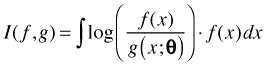
Here f and g are probability distributions and θ denotes the various parameters used in the specification of g. I(f, g) has two equivalent interpretations.
Typically, g is taken to be an approximating model while f is taken to be the true state of nature. As a measure of distance, I(f, g) is a strange beast. Because of the asymmetry in the way f and g are treated in the integral, I(f, g) ≠ I(g, f).
Now suppose we have a second approximating model h that depends on a different parameter set ψ. The K-L information between the true state of nature f and model h is defined as follows.
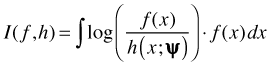
If it turns out that I(f, h) < I(f, g) then we should prefer model h to model g because it is closer to the true state of nature f. Of course all of this ignores an obvious problem. We don't know the true state of nature f and therefore we can't calculate I(f, g) or I(f, h). Fortunately we don't need to know the true state of nature f for these ideas to be useful.
In Fig. 1 models f, g, and h are positioned on their Kullback-Leibler scale so that the vertical distance between f and g is their K-L distance, and the vertical distance between f and h is their K-L distance. Of course we can never actually locate f in this picture (because f is unknown to us), but suppose it is possible to approximate the vertical positions (y-coordinates) of g and h relative to the y = 0 axis. As Fig. 1 shows, the model with the smaller y-coordinate will necessarily be closer to f. Thus we can use the y-coordinates of the models as a way to choose between them. We don't need to know the location of f in Fig. 1, just the relative positions of g and h with respect to each other.
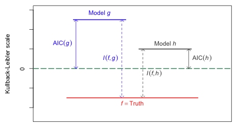 |
| Fig. 1 The connection between AIC and K-L information. While the magnitude of K-L information is interpretable, the magnitude of AIC tells us nothing about the absolute quality of a model. AIC only provides relative information. (R code) |
Akaike (1971) showed that AIC provides an approximate estimate of the relative position of models with respect to their K-L information. Models that have smaller values of AIC are better models than comparable models with larger values of AIC. Because AIC is only a relative measure its numerical value is meaningless. In Fig. 1 we see that AIC is measured with respect to numerical zero rather than to the absolute zero, which in the figure corresponds to the true state of nature. Because its reference point is arbitrary, the absolute magnitude of AIC is not interpretable.
AIC is typically positive, although it can be negative. If the likelihood is constructed from a discrete probability model, the individual terms in the log-likelihood will be log probabilities. These are negative because probabilities are numbers between 0 and 1. AIC multiplies these terms by –2 and hence AIC will be positive for discrete probability models. In continuous probability models the terms of the log-likelihood are log densities. Because a probability density can exceed one AIC can be negative or positive.
Caveat 1. AIC can only be used to compare models that are fit using exactly the same set of observations. This fact can cause problems when fitting regression models to different sets of variables if there are missing values in the data. Consider the following data set consisting of five observations and three variables where one of the variables has a missing value (NA) for observation 3.
| Observation | y | x1 | x2 |
1 |
– |
– |
– |
2 |
– |
– |
– |
3 |
– |
– |
NA |
4 |
– |
– |
– |
5 |
– |
– |
– |
Most regression packages carry out case-wise deletion so that observations with missing values in any of the variables that are used in the model are deleted automatically. Thus in fitting the following three models to these data, the number of available observations will vary.
Model |
Formula |
n |
1 |
y ~ x1 |
5 |
2 |
y ~ x2 |
4 |
3 |
y ~ x1 + x2 |
4 |
Models 2 and 3 being fit to the same four observations are comparable using AIC, but neither of these models can be compared to the AIC of Model 1 which is based on one additional observation. The solution is to delete observation 3 and fit all three models using only the four complete observations 1, 2, 4, and 5. If model 1 ranks best among these three models then model 1 can be refit with observation 3 included.
Because many regression functions do not explicitly warn you that observations have been deleted you need to check this possibility before you begin fitting models. In the rikz data set we were fitting models to richness that involved the predictors NAP and week.
To check for missing values we can use the apply function along with is.na to count the number of missing values in the variables of interest for each observation. The exclamation point, !, is the "not" symbol in R, so !is.na(x) checks whether a variable is not missing (evaluates to TRUE) for a given observation. We then sum this to obtain the number of non-missing values for that observation.
We see that all 45 observations have non-missing values for all three of the variables. Consequently any model we fit involving one or more of these variables can be compared using AIC.
Caveat 2. The response variable must be the same in each model being compared. Monotonic transformations alter the probability densities at individual points in order that the probabilities over intervals remain the same. The likelihood on the other hand only includes the densities at individual points. This means that the log-likelihoods and AICs of models with a transformed response, e.g. log y, cannot be directly compared to the log-likelihoods and AICs of models that are fit to the raw response, y. Fortunately there are ways around this problem.
![]()
The likelihood for the transformed model is
To calculate probabilities we have to integrate the density.
![]()
If you make the substitution
the integral becomes the following.
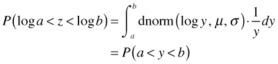
The integrand is now a density on the scale of the response and can be used to construct a likelihood on the scale of the response.
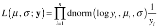
This likelihood is now comparable to other likelihoods that model the raw response y. If y is discrete then each term in this expression can be viewed as the midpoint approximation to the area under the curve over the interval
so that the likelihood can be interpreted as a probability (lecture 8).

This approach is preferable to using the midpoint approximation particularly if there are any observed zeros that make it necessary to add a constant to the response variable before carrying out the transformation (such as log). In this case the above formula has to be modified slightly because the zero values are boundary values and therefore only contribute the first term in the difference to the likelihood.
I fit the three normal and three Poisson models to the richness variable in the rikz data set that we've considered previously.
The AIC function calculates the AIC of each of these models.
So based on AIC we should prefer the interaction model in which richness is assumed to have a Poisson distribution. When using AIC to compare models one should report the log-likelihood, number of estimated parameters, and AIC of each model separately.
Log-transforming count data and assuming the result has a normal distribution has historically been the recommended way to analyze count data particularly if the count distribution is highly skewed. Because there are zero values of richness in the rikz data set, the log transformation is undefined.
The usual "fix" is to add a small constant, 0.5 or 1, to all the observations in the data set before carrying out the transformation. The choice of constant can make a difference in the results.
The reported log-likelihood and AIC would seem to suggest that the log-transformed model handily beats all the models fit thus far. This conclusion is not necessarily correct because the reported log-likelihood is not comparable to the log-likelihoods obtained from fitting models to the raw response. We first need to make one of the adjustments to the likelihood described in the previous section. Using the second method the corrected log-likelihood for the log-transformed model fit above is –109.0533 and the AIC is 224.1067. We'll see how to carry out this adjustment for a different data set in the next lecture.
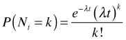
A Poisson random variable is discrete and the Poisson distribution is a standard probability model for count data.The Poisson distribution is bounded below by 0, but is theoretically unbounded above. This distinguishes it from another distribution, the binomial distribution, which is bounded on both sides. The Poisson distribution is a one-parameter distribution. The parameter is usually denoted with the symbol λ and is called the rate of the process.
The mean of the Poisson distribution is equal to the rate, λ. The variance of the Poisson distribution is also equal to λ. Thus in the Poisson distribution the variance is equal to the mean. So if ![]() then
then
Mean:
Variance:
So in the Poisson distribution the variance is a function of the mean, i.e., ![]() . When the mean gets larger, the variance gets larger at exactly the same rate. Contrast this with the normal distribution where the variance is constant and is independent of the mean.
. When the mean gets larger, the variance gets larger at exactly the same rate. Contrast this with the normal distribution where the variance is constant and is independent of the mean.
The Poisson distribution can be derived from three basic assumptions about the underlying process that is generating the data.
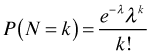
Let ![]() where Nt is the number of events occurring in a time interval of length t, then the probability of observing k events in that interval is
where Nt is the number of events occurring in a time interval of length t, then the probability of observing k events in that interval is
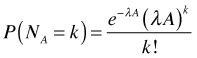
The Poisson distribution can be applied to both time and space. In a Poisson model of two-dimensional space, events occur again at a constant rate such that the number of events observed in an area A is expected on average to be λA. In this case the probability mass function is
For spatial distributions the Poisson distribution plays a role in defining what’s called CSR—complete spatial randomness.
Sometimes we fix the time interval or the area for all observations. If all the quadrats are the same size then we don't need to know what A is. In such cases we suppress t and A in our formula for the probability mass function and write instead
In R the above probability would be calculated as dpois(k, λ).
Unlike some probability distributions that are used largely because they resemble distributions seen in nature, but otherwise have no particular theoretical motivation, the use of the Poisson distribution can be motivated by theory. The Poisson distribution arises in practice in two distinct ways.
| Jack Weiss Phone: (919) 962-5930 E-Mail: jack_weiss@unc.edu Address: Curriculum for the Environment and Ecology, Box 3275, University of North Carolina, Chapel Hill, 27599 Copyright © 2012 Last Revised--February 5, 2012 URL: https://sakai.unc.edu/access/content/group/2842013b-58f5-4453-aa8d-3e01bacbfc3d/public/Ecol562_Spring2012/docs/lectures/lecture10.htm |