Today we continue our discussion of maximum likelihood estimation by using it to obtain parameter estimates of a Poisson regression model. We start by constructing the likelihood from first principles, then plot the log-likelihood to determine the maximum likelihood estimate (MLE) graphically, and finally use R's optimization functions to obtain the estimate numerically. Poisson regression models can also be fit using the glm function of R. The summary, anova, coef, and predict functions when used on glm objects produce output similar to what we obtained using lm. To compare Poisson regression models to their normal regression model counterparts we use three-dimensional graphics and analytical methods. Finally a graphical method is used to assess the fit of a Poisson regression model.
The Rikz data set is a supposedly random sample of m = 45 sites that we've used to construct regression models for species richness at the sites. When we regressed richness against NAP we saw problems with the underlying assumption that the response variable is normally distributed about the regression line with constant variance. In particular the model predicted that at large NAP values, but still within the range of the data, there is a sizable probability for richness values generated by the model to be negative.
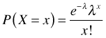
The problem with using a normal distribution for these data is that it doesn't respect the natural characteristics of the data. A normally distributed response is a continuous variable but richness can assume only non-negative integer values. An alternative probability model that is often used with count data is the Poisson distribution whose probability mass function is
In R the Poisson probability mass function is given by dpois(x, lambda).
In lecture 7 we showed that if we have a random sample then the joint probability of our data can be written as follows.
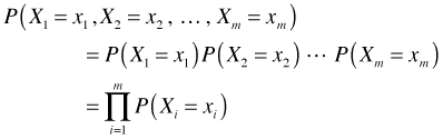
Plugging Poisson probabilities into our expression for the joint probability yields the following.
where in the last step the joint probability is denoted by f, a function of the data (x1, x2, ... , xm) as well as the Poisson parameter λ. If we knew λ then we could calculate the probability of obtaining any set of observed values x1, x2, ... , xm. Furthermore, for fixed λ if we summed this expression over all possible values of x1, x2, ... , xm we would get 1, because f is a probability function.
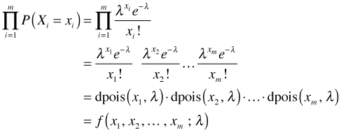
In Poisson regression we typically model the rate parameter λ of the Poisson distribution in terms of predictors. For reasons we'll explain later the preferred approach is to model log λ rather than λ.
So under this scenario the probability of our data would be the following.
where xi is the observed species richness in sample i.
Typically when using a probability distribution such as the Poisson we think of the parameters as fixed and the data as random. Given fixed values of the parameters, the Poisson formula returns the probability of obtaining a specific data value. In likelihood theory we turn these roles around. We view the data as fixed (after all, it's been collected so it's no longer random) and the parameters as random. To emphasize this in the Poisson example we could write the probability of our data as follows.
![]()
where we now use the symbol L instead of f and we switch the order of its arguments. Viewed this way L is not a a probability. For fixed data if we sum over all possible values of λ we will not get 1. So when we think of the probability function as a function of the parameters rather than a function of the data we call it a likelihood. If we plug in values for λ we get different values for the likelihood. Keep in mind that fundamentally it is still the joint probability function for our data under the assumed probability model, only by another name.
From a likelihood perspective a natural question to ask is the following, is there a value of λ at which the likelihood achieves a maximum? Or, put another way, is there a value of λ that makes obtaining the data we actually obtained most probable? In terms of our regression problem above we seek the values of β0 and β1 that make it most likely to obtain the data we actually obtained. We call those parameter values the maximum likelihood estimates (MLEs) of the parameters, because they maximize the likelihood. One of R. A. Fisher's major contributions to statistics (among many) was to realize that the likelihood function is a vehicle for obtaining parameter estimates.
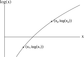
Fig. 1 Monotonicity of the logarithm function
For both practical and theoretical reasons it is preferable to work with the log of the likelihood rather than the likelihood itself. Because the logarithm of a product is the sum of the logs, the log-likelihood has a simpler form than does the likelihood.

or for our Poisson example
If our goal is to find the values of the parameters that maximize the likelihood, then nothing is lost if we choose to maximize the log-likelihood instead. This is because the logarithm function is a monotone increasing function. In other words if x1 < x2 it also must be the case that log(x1) < log(x2), and vice versa (Fig. 1). Consequently in our Poisson example the monotonicity of the logarithm function means that the value of λ that maximizes log L is also the value of λ that maximizes L.
We begin by loading the Rikz data set and refitting some of the normal models from before.
The Poisson distribution is a standard model for non-negative discrete data (counts). The Poisson distribution is defined by a single parameter called the rate of the process that is generally denoted by the Greek letter λ. We start with a simple Poisson model in which we assume a constant value for λ. This is equivalent to a regression model in which we fit only an intercept.
The expression for the Poisson log-likelihood given at the end of the last section can be translated directly into R language as follows.
The dpois function is listable. Thus for a fixed value of λ we can obtain the probabilities for all of our richness observations at once. Let's study the behavior of the log-likelihood for different values for λ.
Remember our goal is to maximize the log-likelihood. Because we are dealing with probabilities the log-likelihood is negative and so we're looking for the least negative value of the log-likelihood. Thus if we had to pick a value for λ among the six we've examined so far, we should choose λ = 6, because it produced the largest value of the log-likelihood. If the log-likelihood is well-behaved then it would seem that the log-likelihood is maximized somewhere between λ = 5 and λ = 7.
What happens if we try to evaluate our function on a vector of values?
It returns a single number that is neither the log-likelihood at λ = 4 nor the log-likelihood at λ = 5. What gives? In the Poisson.LL function dpois is given a vector first argument, rikz$richness, that is of length 45. With 4:5 we are passing a vector of length 2 to dpois for its second argument lambda. When a listable R function is given two vector arguments of different lengths it tries to match them up and, if necessary, it recycles the values of the shorter one until it is the same length as the longer one. Thus R creates the vector 4, 5, 4, 5, ... and uses this for its lambda argument. As a result we get the log Poisson probability of the first observation using lambda = 4, the log Poisson probability of the second observation using lambda = 5, the log Poisson probability of the third observation using lambda = 4, etc. The values of lambda alternate between 4 and 5 each time and the result is nonsensical expression.
The solution to this is to force R to use each element of the lambda argument once for all the values of rikz$richness before moving onto the next element of lambda. The sapply function can be used to do this. The sapply function will force the function that is given as its second argument to be evaluated separately for each element of its first argument.
Now we get what we want: the log-likelihood evaluated once for λ = 4 and a second time for λ = 5.
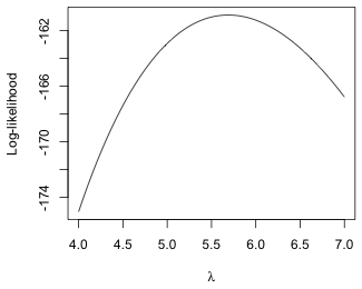
Fig. 2 Plot of the log-likelihood function
To graph the log-likelihood we can evaluate our function on a whole list of possible values of λ and then plot the results against λ. For example to plot over the domain 4 ≤ λ ≤ 7, we could first generate λ in increments of 0.01 with seq(4,7,.01) to use as the x-coordinates and then sapply the Poisson log-likelihood function to this vector of numbers to generate the corresponding function values for the y-coordinates.
plot(seq(4, 7, .01), sapply(seq(4, 7, .01), Poisson.LL), type='l', ylab='Log-likelihood', xlab=expression(lambda))
From Fig. 2 we see that the maximum of the log-likelihood occurs somewhere between 5.5 and 6.0.
Clearly we could repeatedly zoom in on the MLE graphically and obtain an estimate that is as accurate as we please, but such an approach is tedious and unwieldy. It is far more efficient to obtain the estimate using numerical optimization. R provides three numerical optimization functions that are useful here, nlm, nlminb, and optim (including its one-dimensional version optimize). Since the current problem is one-dimensional we use optimize. The help screen for optimize indicates that we need to specify three arguments: the function to optimize, an interval over which to search for the optimum value, and the argument maximum=T to indicate that we want a maximum value rather than a minimum value. Since we've already seen that the interval (4, 7) brackets the maximum we use this interval as the search interval.
$objective
[1] -160.8757
The reported maximum value of the log-likelihood is –160.88 and it occurs at λ = 5.69.
One change we can make to the current model is to allow each site to have its own rate parameter. We begin by letting the Poisson parameter λ vary with a site's value of NAP. Because the rate parameter is also the mean of the Poisson distribution this is equivalent to constructing a regression model for the mean.
![]()
The function for constructing the log-likelihood under this scenario is displayed below. It's a multi-lined function in which the first line defines the Poisson mean and the second line then uses it as the lambda argument of the dpois function.
The optimization functions of R only accepts single parameter arguments. In order to fit models with multiple parameters we must make these parameters the components of a vector. Here the vector is denoted by x and it has length 2. The first component x[1] is the intercept and the second component x[2] is the slope in the regression equation. As a result when we use this function we have to supply it a vector of length 2.
In order to use the optimization functions of R to obtain the MLE we first need initial estimates of the components of x.
This choice apparently produced some illegal values for the Poisson parameter λ. The reason this happened is because we are using an identity link which offers no protection against the parameter being negative. A log link would be a better choice here.
Because (7, –3) yields a larger log-likelihood than (7, –2) we use its components for the starting values.
All of the R optimization functions carry out minimization instead of maximization. Thus in order for us to be able to use them we need to change the way we've been formulating the problem. Since maximizing a function f is equivalent to minimizing a function –f, we need to re-express our objective function so that it returns the negative log-likelihood rather than the log-likelihood.
The optim function expects a vector of initial guesses as the first argument and the function to be minimized as the second argument.
$value
[1] 122.2139
$counts
function gradient
49 NA
$convergence
[1] 0
$message
NULL
Warning messages:
1: In dpois(x, lambda, log) : NaNs produced
2: In dpois(x, lambda, log) : NaNs produced
3: In dpois(x, lambda, log) : NaNs produced
4: In dpois(x, lambda, log) : NaNs produced
5: In dpois(x, lambda, log) : NaNs produced
The output tells us the following.
A second optimization function in R is the nlm function. It also does minimization but it expects the arguments to be in the reverse order from optim: first the function to be minimized and second the initial guesses for the parameters in the form of a vector.
$estimate
[1] 6.693129 -2.888344
$gradient
[1] -7.237990e-06 -5.018472e-06
$code
[1] 1
$iterations
[1] 8
Warning messages:
1: In dpois(x, lambda, log) : NaNs produced
2: In nlm(neg.LL, c(7, -3)) : NA/Inf replaced by maximum positive value
3: In dpois(x, lambda, log) : NaNs produced
4: In nlm(neg.LL, c(7, -3)) : NA/Inf replaced by maximum positive value
The output tells us the following.
The warning messages indicate that problems arose during the iterations but that both optim and nlm managed to recover from them. These problems occurred because we fit a model using an identity link, which failed to prevent the Poisson mean from becoming negative. To correct this we refit the same model using a log link.
To improve numerical stability and prevent the iterations from generating illegal values for the Poisson mean, we rewrite the log-likelihood function using a log link. With a log link the regression model is
![]()
The corresponding R function is the following.
Notice that the log link is exponentiated when it's entered as the second argument to dpois. As before we need to experiment with the function to obtain good starting values for the parameters.
The largest value of the log-likelihood is obtained with β0 = 2, β1 = 0.25 so we can use these as our initial guesses. This time we construct the negative log-likelihood function on the fly using a generic function as the second argument to optim.
$value
[1] 127.5904
$counts
function gradient
57 NA
$convergence
[1] 0
$message
NULL
Now we get numerical convergence without any warning messages. The solution this time is β0 = 1.791, β1 = –0.556.
Regression models in which the response has a Poisson distribution are easily fit with the glm function of R. The glm function supports additional probability distributions for the response besides the Poisson. These distributions are connected in that they are all members of what's called the exponential family of probability distributions. We'll discuss some of these other distributions later.
The syntax of glm is identical to that of lm except that glm accepts an optional family argument that can be used to specify the desired probability distribution. If the family argument is not specified then glm uses a normal distribution. To fit a Poisson regression model with richness as the response and NAP as the predictor we would proceed as follows. A log link for the mean is the default in Poisson regression and doesn't have to be specifically requested.
The summary and anova functions can be used on a glm object to obtain statistical tests. For anova we need to specify an additional argument, test='Chisq', in order to get p-values for the reported statistical tests.
Model: poisson, link: log
Response: richness
Terms added sequentially (first to last)
Df Deviance Resid. Df Resid. Dev Pr(>Chi)
NULL 44 179.75
NAP 1 66.571 43 113.18 3.376e-16 ***
---
Signif. codes: 0 ‘***’ 0.001 ‘**’ 0.01 ‘*’ 0.05 ‘.’ 0.1 ‘ ’ 1
Deviance Residuals:
Min 1Q Median 3Q Max
-2.2029 -1.2432 -0.9199 0.3943 4.3256
Coefficients:
Estimate Std. Error z value Pr(>|z|)
(Intercept) 1.79100 0.06329 28.297 < 2e-16 ***
NAP -0.55597 0.07163 -7.762 8.39e-15 ***
---
Signif. codes: 0 ‘***’ 0.001 ‘**’ 0.01 ‘*’ 0.05 ‘.’ 0.1 ‘ ’ 1
(Dispersion parameter for poisson family taken to be 1)
Null deviance: 179.75 on 44 degrees of freedom
Residual deviance: 113.18 on 43 degrees of freedom
AIC: 259.18
Number of Fisher Scoring iterations: 5
From the output we learn that the estimated regression equation is log μ = 1.791 – 0.556*NAP. This matches what we obtained with the optim function in the previous section.
Although some of the language used in the output will appear strange, e.g., use of the word 'deviance', the output itself should seem familiar. The anova function carries out a sequence of tests on nested models whereas the summary table reports variables-added-last tests. Formally, the anova output reports the results from likelihood ratio tests (analogous to the F-tests of ordinary regression) whereas the summary table reports the results from Wald tests (analogous to the t-tests of ordinary regression). In ordinary regression the t-tests and F-tests are mathematically related and when they are testing the same hypothesis they give the same results. In the likelihood framework, the likelihood ratio tests and Wald tests are constructed from different assumptions and will typically give different results even when they are testing the same hypothesis. This is the case in the above tables where both are testing the hypothesis H0: β1 = 0, but the reported p-values are slightly different.
To fit a Poisson regression model with an identity link we need to specify the link as part of the family argument.
The model returns an error message because the built-in algorithm generated starting values that caused problems for the optimization routine. This situation is not unusual when using link functions that are different from the default. We need to supply our own initial values just as we did with the optim function. For glm these are supplied in a start argument.
The values supplied didn't work so we try again.
Curiously these starting values worked even though they are much farther away from the final solution than the first choice of 6 and –3 are.
If we give it starting values very close to the true solution it also converges to a solution.
From the output of the coef function, the estimated regression model with an identity link is the following: μ = 6.693 – 2.888*NAP.
We can compare the log-likelihoods of the two models we've fit, one using a log link and the other using an identity link, and see which model makes the data more probable. The logLik function of R extracts log-likelihoods from glm objects.
The log-likelihood of the Poisson model with an identity link is larger suggesting it provides a better fit to the data. To extract the log-likelihoods of both models with a single function call we need to use the sapply function and the list function to group the two models together.
[1] -127.5904 -122.2139
The predict function when applied to a glm object returns predictions on the scale of the link function. So when we apply it to the glm model object mod1p in which we used a log link, it returns estimates of log μ for each observation.
To obtain estimates of μ we can just exponentiate these values, or alternatively, use the fitted function. The fitted function returns predictions on the scale of the response, i.e., it also inverts the link function.
In lecture 7 we generated a three-dimensional picture of the normal regression model and saw that the normal model had some problems with it. It would be useful to produce the same graph for the two Poisson models that we've considered, a model with a log link and a model with an identity link, and see how they compare. For that we need to make only trivial modifications to the code from lecture 7. The code is shown below with the changes highlighted in blue.
 |
|
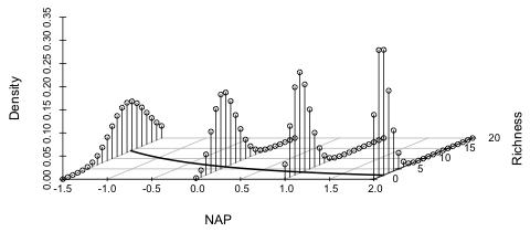
| Fig. 3 Poisson regression model using a log link | |
The distributions are plotted as bar graphs rather than curves because the Poisson distribution is only defined at non-negative integer values. Observe how the regression "line" curves around and comes in asymptotic to the NAP-axis. Notice also that when the Poisson mean is far removed from zero, the Poisson distribution is symmetric (e.g., at NAP = –1.5), but as the mean gets closer to zero the Poisson distribution becomes positively skewed.
To produce this graph for the Poisson model with an identity link requires only changing the expressions for mu and mu2 in the above code.
 |
|
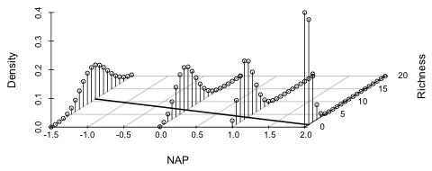
| Fig. 4 Poisson regression model using an identity link | |
Although the model with an identity link yielded a larger log-likelihood than did the Poisson model with a log link, it's clear in Fig. 4 that extending the regression line to larger NAP values will cause it to eventually cross the x-axis and predict negative values for mean richness. Thus we might prefer the log link model here because it is generalizable to new data.
We can also fit Poisson regression model versions of the ordinary regression models we fit to these data previously. The next two models add week as a categorical variable.
To test these models we can use the anova function on the interaction model.
Model: poisson, link: log
Response: richness
Terms added sequentially (first to last)
Df Deviance Resid. Df Resid. Dev Pr(>Chi)
NULL 44 179.753
NAP 1 66.571 43 113.182 3.376e-16 ***
factor(week) 3 59.716 40 53.466 6.759e-13 ***
NAP:factor(week) 3 22.396 37 31.070 5.396e-05 ***
---
Signif. codes: 0 ‘***’ 0.001 ‘**’ 0.01 ‘*’ 0.05 ‘.’ 0.1 ‘ ’ 1
The output is interpreted the same way as the ANOVA table for ordinary regression. The NULL model that appears first is one that contains only an intercept. The second line tells us that adding NAP is a significant improvement over the intercept-only model. Line 3 tells us that adding week to the NAP model yields a significant improvement. Line 4 tells us that adding the NAP × week interaction to the NAP + week model yields a significant improvement. Thus our final Poisson regression model should be the interaction model where the effect of NAP varies by week. Using the summary table we can then determine the nature of the interaction just as we did with the normal model.
We can use the magnitudes of the log-likelihoods to compare the final Poisson model with the final normal model.
Because the log-likelihood of the Poisson model exceeds that of the normal model, we would like to argue that the Poisson model is preferable—the data are more likely under the Poisson model than under the normal model. This remark needs further justification. Because the normal likelihood is a product of densities (which don't have an immediate probability interpretation) whereas the Poisson likelihood is a product of probability mass functions (which do have a probability interpretation), it's not at all clear that these two likelihoods are comparable.
Because of the central limit theorem and the fact that the normal distribution provides a decent approximation to many probability models, it is perfectly legitimate to use the normal distribution, a model that assumes an underlying continuum, even when a variable is discrete. Even more common is the practice of log-transforming or square-root transforming a discrete response variable and then assuming the result is normally distributed. As a result it would be nice to have a direct way to compare the likelihoods derived from discrete and continuous probability models when applied to the same data set.
At first glance this would not seem to be possible because likelihoods based on continuous probability models are densities while those based on discrete probability models are probabilities. To obtain a probability from a density requires integrating that density over an interval. In particular if X is a continuous random variable, then ![]() for all values of k. It is only expressions of the form
for all values of k. It is only expressions of the form ![]() , for some interval (a, b), that can have nonzero values.
, for some interval (a, b), that can have nonzero values.
Obviously we do use continuous probability models for discrete random variables, so what does an expression of the form P(X = k) mean when k can only take non-negative integer values? The standard interpretation is the following.
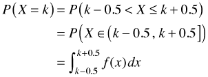
and so we have an implicit interval over which we can integrate the density. (Whether the interval is defined to be open, closed, or half-open is immaterial here.) Notice that the interval in question has length = 1 and that the value X = k is the midpoint of this interval. The midpoint rule for approximating an integral tells us that
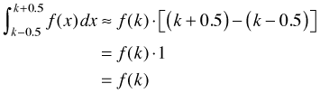
which is just the density. Thus we see that any density used as a model for discrete data can be interpreted as a probability in the approximating sense of the midpoint rule.

Fig. 5 Using a continuous density to approximate a discrete probability (R code)
Fig. 5 displays the predicted normal distribution for observation #4 using the NAP × week interaction model. The observed richness for observation #4 is 11. Because the normal distribution is continuous, calculating P(X = 11) requires evaluating the following integral.
![]()
where ![]() is the normal density predicted for observation #4. The graph on the left in Fig. 5 displays the midpoint approximation for this integral, the area of a rectangle whose height is the density evaluated at X = 11 and whose width is 1. So, an approximate value of P(X = 11) is just the density evaluated at X = 11. The normal density function in R is dnorm.
is the normal density predicted for observation #4. The graph on the left in Fig. 5 displays the midpoint approximation for this integral, the area of a rectangle whose height is the density evaluated at X = 11 and whose width is 1. So, an approximate value of P(X = 11) is just the density evaluated at X = 11. The normal density function in R is dnorm.
The graph on the right in Fig. 5 displays the exact value of P(X = 11), the true area underneath the density curve from x = 10.5 to x = 11.5. The pnorm function in R is the normal cumulative distribution function. It returns the following value.
![]()
This is the area under the graph from x = –∞ to x = a. Thus we can find the area under the graph from x = a to x = b by subtracting pnorm(a,μ,σ) from pnorm(b,μ,σ). For our example b = 11.5 and a = 10.5 as is shown at the top of the figure.
To carry out these calculations in R the predict function is used to extract the estimated mean of the normal distribution for observation #4.
The estimated mean and standard deviation of the normal distribution can be used to calculate P(X = 11), first using the midpoint approximation and then using the exact formula.
The answers agree to the second decimal place. Next we compare the exact and approximate probabilities for all 45 observations.
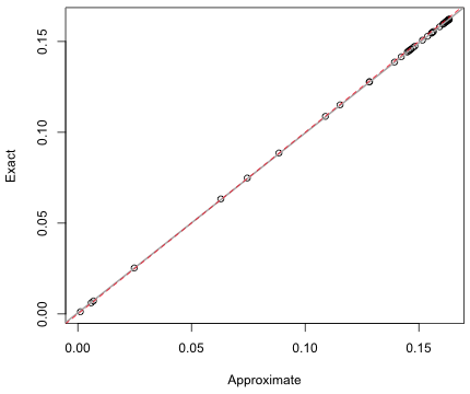
Fig. 6 Comparing exact and approximate normal probabilities
The approximate and exact probabilities shown in Fig. 6 appear to be exceptionally close. In reality the approximate probability consistently overestimates the true probability by a small amount. If we construct a 95% confidence interval for the slope we see that it doesn't include 1, so we would reject the hypothesis that the two probabilities are equal.
The Poisson regression model estimates the mean of a Poisson distribution for each observation. Using it we can then construct the corresponding probability distribution of a Poisson random variable with that mean. To check the fit of the model we can assess whether the observed richness values look as if they could have arisen from their predicted distributions.
We begin by calculating the Poisson probabilities of X = 0 up to and including X = 30 for each observation in the Rikz data set. Because we need to carry out this calculation separately for each observation we use the sapply function.
From the dimensions of the output we can tell that the columns correspond to the different probabilities and the rows correspond to the different observations.
We need to unstack this matrix into a single vector so it can be incorporated into a data frame. The as.vector function converts a matrix into a vector by stacking the columns of the matrix one on top of the other. To keep probabilities from individual observations together we first transpose the matrix using the R t function, which swaps rows and columns, before using the as.vector function.
In addition to the probabilities we need the following.
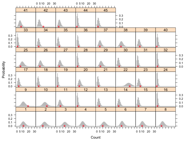
Next we construct a panel graph showing the 45 sites in separate panels. Each panel displays the predicted Poisson distribution as a bar plot (using panel.xyplot and type='h' to drop vertical lines to the x-axis) with the observed count superimposed on this distribution to see if it looks typical.
 |
|
| Fig. 7 Panel graph of the predicted Poisson distributions at each site. The observed richness (*) is shown relative to its predicted distribution. | |
Most of the distributions are compressed because we're displaying more probabilities than are necessary. The smallest probability of an actual observation is 0.003,
so we can remove all probabilities less than 0.001 and redo the plot. The x-axis is made 'free' so that the x-limits in each panel are adjusted according to what is being displayed.
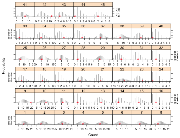
Fig. 8 A repetition of Fig. 6 in which negligible tail probabilities have been removed.
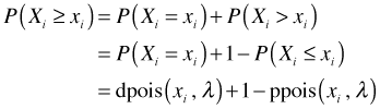
The only sites in which the observed richness count appears to be an outlier are sites 9 and 42. We can quantify this further by calculating a p-value for the observed richness in each site. The p-value is a tail probability, the probability of observing a value as extreme or more extreme than what was actually observed. We focus on the upper-tail p-values because its clear that there are no lower-tailed outliers. If xi is the observed richness value in site i then the p-value can be calculated as follows.
The only p-values less than 0.05 correspond to site 9 (p = 0.02) and site 42 (p = 0.005). With 45 sites we'd expect to obtain .05*45 = 2.25 significant p-values by chance alone, so what we obtained is not an unusual result. We conclude that the observed richness counts could very well have arisen from the proposed model.
| Jack Weiss Phone: (919) 962-5930 E-Mail: jack_weiss@unc.edu Address: Curriculum for the Environment and Ecology, Box 3275, University of North Carolina, Chapel Hill, 27599 Copyright © 2012 Last Revised--Jan 31, 2012 URL: https://sakai.unc.edu/access/content/group/2842013b-58f5-4453-aa8d-3e01bacbfc3d/public/Ecol562_Spring2012/docs/lectures/lecture8.htm |