Assignment 7—Solution
Question 1
pyrau <- read.delim('Pyrausta.txt')
pyrau
eggs X1936 X1937 X1938
1 0 26 37 14
2 1 19 14 21
3 2 7 2 11
4 3 1 3 7
5 4 3 0 2
I begin by converting the tabulated data into raw data. For this I use the rep function once for each year. In each case I rep the eggs column by the frequencies that appear in the year columns.
y.1936 <- rep(pyrau$eggs, pyrau$X1936)
y.1937 <- rep(pyrau$eggs, pyrau$X1937)
y.1938 <- rep(pyrau$eggs, pyrau$X1938)
Next I concatenate these three vectors together and make them a column in a data frame. To create a year variable I rep each year by the total for that year (obtained by taking the length of raw data vector for that year) and turn the result into a factor.
pyrau.raw <- data.frame(count=c(y.1936, y.1937, y.1938), year=factor(rep(1936:1938, c(length(y.1936), length(y.1937), length(y.1938)))))
dim(pyrau.raw)
[1] 167 2
Using glm
To test for a year effect I use glm to fit a Poisson regression model in which year is the only predictor. I use the anova function to carry out a likelihood ratio test for the effect of year.
out1 <- glm(count~year, data=pyrau.raw, family=poisson)
anova(out1, test='Chisq')
Analysis of Deviance Table
Model: poisson, link: log
Response: count
Terms added sequentially (first to last)
>
Df Deviance Resid. Df Resid. Dev Pr(>Chi)
NULL 166 220.91
year 2 22.095 164 198.82 1.593e-05 ***
---
Signif. codes: 0 ‘***’ 0.001 ‘**’ 0.01 ‘*’ 0.05 ‘.’ 0.1 ‘ ’ 1
The model being fit is the following.

The likelihood ratio test tests the following hypothesis.
H0: β1 = β2 = 0
H1: at least one of β1, β2 not zero
The reported p-value for the test is small so we reject the null hypothesis and conclude there is a year effect. If we examine the summary table we can determine how the years differ.
summary(out1)
Call:
glm(formula = count ~ year, family = poisson, data = pyrau.raw)
Deviance Residuals:
Min 1Q Median 3Q Max
-1.6181 -0.9820 -0.2820 0.5599 2.4572
Coefficients:
Estimate Std. Error z value Pr(>|z|)
(Intercept) -0.1542 0.1443 -1.068 0.2855
year1937 -0.5754 0.2406 -2.392 0.0168 *
year1938 0.4235 0.1863 2.273 0.0230 *
---
Signif. codes: 0 ‘***’ 0.001 ‘**’ 0.01 ‘*’ 0.05 ‘.’ 0.1 ‘ ’ 1
(Dispersion parameter for poisson family taken to be 1)
Null deviance: 220.91 on 166 degrees of freedom
Residual deviance: 198.82 on 164 degrees of freedom
AIC: 414.33
Number of Fisher Scoring iterations: 6
From the output we see that the mean in 1937 is significantly lower than the mean in 1936 (the reference group) and the mean in 1938 is significantly higher than the mean in 1936. Given this and the fact that the means are ranked  , it follows that the means in 1937 and 1938 are also significantly different. Thus all the means differ from each other.
Using nlm
Alternatively we can construct the log-likelihoods ourselves and use nlm to obtain the maximum likelihood estimates and to carry out the likelihood ratio test.
# common mean model
negpois1.LL <- function(p){
LL <- sum(log(dpois(pyrau.raw$count, lambda=p)))
-LL
}
out.pois1 <- nlm(negpois1.LL,.8)
out.pois1
# separate means model
negpois2.LL <- function(p){
mu <- p[1] + p[2]*(pyrau.raw$year==1937) + p[3]*(pyrau.raw$year==1938)
LL <- sum(log(dpois(pyrau.raw$count, lambda=mu)))
-LL
}
out.pois2 <- nlm(negpois2.LL, c(0.8,-0.4,0.4))
LRstat <- 2*(out.pois1$minimum-out.pois2$minimum)
LRstat
[1] 22.09468
length(out.pois2$estimate)-length(out.pois1$estimate)
[1] 2
1-pchisq(LRstat, df=2)
[1] 1.592949e-05
This is the same answer we obtained with the anova function on the glm object.
Question 2
We need the tabulated data for the plot. I rep the count categories three times, concatenate the three columns of frequencies together, and make a third column that records the year.
pyrau.table <- data.frame(count=rep(pyrau$eggs,3), freq=unlist(pyrau[,2:4]), year=factor(rep(1936:1938, each=5)))
rownames(pyrau.table) <- NULL
pyrau.table
count freq year
1 0 26 1936
2 1 19 1936
3 2 7 1936
4 3 1 1936
5 4 3 1936
6 0 37 1937
7 1 14 1937
8 2 2 1937
9 3 3 1937
10 4 0 1937
11 0 14 1938
12 1 21 1938
13 2 11 1938
14 3 7 1938
15 4 2 1938
I use the predict function with the newdata argument to add the predicted mean for each year to the data frame.
pyrau.table$mu <- predict(out1, type='response', newdata=data.frame(year=pyrau.table$year))
pyrau.table
count freq year mu
1 0 26 1936 0.8571429
2 1 19 1936 0.8571429
3 2 7 1936 0.8571429
4 3 1 1936 0.8571429
5 4 3 1936 0.8571429
6 0 37 1937 0.4821429
7 1 14 1937 0.4821429
8 2 2 1937 0.4821429
9 3 3 1937 0.4821429
10 4 0 1937 0.4821429
11 0 14 1938 1.3090909
12 1 21 1938 1.3090909
13 2 11 1938 1.3090909
14 3 7 1938 1.3090909
15 4 2 1938 1.3090909
Next I use the dpois function to calculate the Poisson probabilities of the count categories using the mean just created. I add the tail probabilities to the last reported category, X = 4.
pyrau.table$p <- dpois(pyrau.table$count, pyrau.table$mu)
pyrau.table$p2 <- pyrau.table$p + ppois(4, pyrau.table$mu, lower.tail=F) * (pyrau.table$count==4)
pyrau.table
count freq year mu p p2
1 0 26 1936 0.8571429 0.424372846 0.424372846
2 1 19 1936 0.8571429 0.363748153 0.363748153
3 2 7 1936 0.8571429 0.155892066 0.155892066
4 3 1 1936 0.8571429 0.044540590 0.044540590
5 4 3 1936 0.8571429 0.009544412 0.011446345
6 0 37 1937 0.4821429 0.617458847 0.617458847
7 1 14 1937 0.4821429 0.297703373 0.297703373
8 2 2 1937 0.4821429 0.071767777 0.071767777
9 3 3 1937 0.4821429 0.011534107 0.011534107
10 4 0 1937 0.4821429 0.001390272 0.001535896
11 0 14 1938 1.3090909 0.270065459 0.270065459
12 1 21 1938 1.3090909 0.353540237 0.353540237
13 2 11 1938 1.3090909 0.231408155 0.231408155
14 3 7 1938 1.3090909 0.100978104 0.100978104
15 4 2 1938 1.3090909 0.033047380 0.044008045
Obtaining the expected counts
Method 1:
To get the expected category counts according to the model we need the count totals for each year.
apply(pyrau[,2:4],2,sum)
X1936 X1937 X1938
56 56 55
A simple way to obtain the expected counts is with an ifelse in which I multiply the probabilities by 55 for year 1938 and by 56 otherwise.
pyrau.table$exp <- ifelse(pyrau.table$year==1938, pyrau.table$p2*55, pyrau.table$p2*56)
pyrau.table
count freq year mu p p2 exp
1 0 26 1936 0.8571429 0.424372846 0.424372846 23.76487936
2 1 19 1936 0.8571429 0.363748153 0.363748153 20.36989659
3 2 7 1936 0.8571429 0.155892066 0.155892066 8.72995568
4 3 1 1936 0.8571429 0.044540590 0.044540590 2.49427305
5 4 3 1936 0.8571429 0.009544412 0.011446345 0.64099531
6 0 37 1937 0.4821429 0.617458847 0.617458847 34.57769544
7 1 14 1937 0.4821429 0.297703373 0.297703373 16.67138887
8 2 2 1937 0.4821429 0.071767777 0.071767777 4.01899553
9 3 3 1937 0.4821429 0.011534107 0.011534107 0.64591000
10 4 0 1937 0.4821429 0.001390272 0.001535896 0.08601017
11 0 14 1938 1.3090909 0.270065459 0.270065459 14.85360024
12 1 21 1938 1.3090909 0.353540237 0.353540237 19.44471304
13 2 11 1938 1.3090909 0.231408155 0.231408155 12.72744853
14 3 7 1938 1.3090909 0.100978104 0.100978104 5.55379572
15 4 2 1938 1.3090909 0.033047380 0.044008045 2.42044246
Method 2:
Use the fact that becausde year is a factor when it gets converted to a numeric variable it has the values 1, 2, and 3. These can then be used to select the correct total from a vector of totals.
n <- apply(pyrau[,2:4], 2, sum)
pyrau.table$exp <- pyrau.table$p2 * n[as.numeric(pyrau.table$year)]
Method 3:
A more general method is to tabulate the counts and collect them in a separate data frame with a year variable. Then using the year variable as the key field we canI do a many-to-one merge and add the sample totals as a new column to the data frame. To get the expected counts multiply the sample total column by the probability column.
n <- apply(pyrau[,2:4], 2, sum)
new.dat <- data.frame(year=1936:1938, n=as.numeric(apply(pyrau[,2:4], 2, sum)))
new.dat
year n
1 1936 56
2 1937 56
3 1938 55
pyrau.table2 <- merge(pyrau.table, new.dat)
pyrau.table2$exp <- pyrau.table2$p2*pyrau.table2$n
pyrau.table2
year count freq mu p p2 n exp
1 1936 0 26 0.8571429 0.424372846 0.424372846 56 23.76487936
2 1936 1 19 0.8571429 0.363748153 0.363748153 56 20.36989659
3 1936 2 7 0.8571429 0.155892066 0.155892066 56 8.72995568
4 1936 3 1 0.8571429 0.044540590 0.044540590 56 2.49427305
5 1936 4 3 0.8571429 0.009544412 0.011446345 56 0.64099531
6 1937 0 37 0.4821429 0.617458847 0.617458847 56 34.57769544
7 1937 1 14 0.4821429 0.297703373 0.297703373 56 16.67138887
8 1937 2 2 0.4821429 0.071767777 0.071767777 56 4.01899553
9 1937 3 3 0.4821429 0.011534107 0.011534107 56 0.64591000
10 1937 4 0 0.4821429 0.001390272 0.001535896 56 0.08601017
11 1938 0 14 1.3090909 0.270065459 0.270065459 55 14.85360024
12 1938 1 21 1.3090909 0.353540237 0.353540237 55 19.44471304
13 1938 2 11 1.3090909 0.231408155 0.231408155 55 12.72744853
14 1938 3 7 1.3090909 0.100978104 0.100978104 55 5.55379572
15 1938 4 2 1.3090909 0.033047380 0.044008045 55 2.42044246
Graph the results
Finally we can produce the graph.
library(lattice)
xyplot(freq~count|year, data=pyrau.table, xlab='Count category', panel=function(x, y, subscripts) {
panel.xyplot(x, y, type='h', lineend=1, col='grey', lwd=10)
panel.points(x, pyrau.table$exp[subscripts], pch=16, cex=.6, col=1, type='o')
}, key=list(x=.82, y=.80, corner=c(0,0), points=list(pch=c(15,16), cex=c(1.2,.7), col=c('grey70', 'black')), text=list(c('observed', 'expected'), cex=.9)))
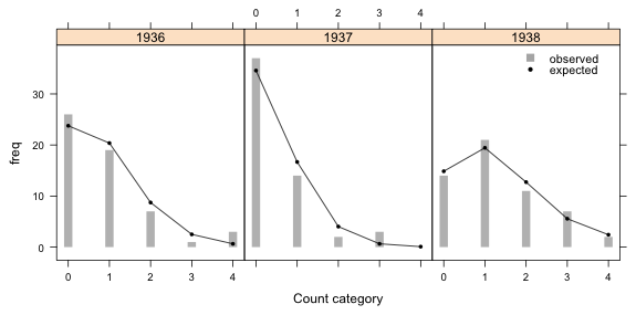
Fig. 1 Predicted and observed count categories under a Poisson model
Question 3
The simplest way to carry out the parametric bootstrap separately by year is with the chisq.test function. We just need to use it three times each time selecting the appropriate observed counts and predicted probabilities for the corresponding year.
chisq.test(pyrau.table$freq[1:5],p=pyrau.table$p2[1:5],simulate.p.value=T, B=9999)
Chi-squared test for given probabilities with simulated p-value
(based on 9999 replicates)
data: pyrau.table$freq[1:5]
X-squared = 10.222, df = NA, p-value = 0.0478
chisq.test(pyrau.table$freq[6:10],p=pyrau.table$p2[6:10],simulate.p.value=T, B=9999)
Chi-squared test for given probabilities with simulated p-value
(based on 9999 replicates)
data: pyrau.table$freq[6:10]
X-squared = 10.2778, df = NA, p-value = 0.1048
chisq.test(pyrau.table$freq[11:15],p=pyrau.table$p2[11:15],simulate.p.value=T, B=9999)
Chi-squared test for given probabilities with simulated p-value
(based on 9999 replicates)
data: pyrau.table$freq[11:15]
X-squared = 0.8575, df = NA, p-value = 0.9332
Based on the output it is only the fit in 1936 that is suspect. To determine what's driving the lack of fit we can look at the individual contributions to the Pearson statistic. Doing so we see that it's the last term corresponding to X = 4 that is the largest. In fact, its contribution is 85% of the entire Pearson statistic. Under the fitted Poisson model observing three counts of four is apparently highly unlikely, yet that is exactly what was observed in 1936.
sum((pyrau.table$freq[1:5] - pyrau.table$exp[1:5])^2/pyrau.table$exp[1:5])
[1] 10.22201
(pyrau.table$freq[1:5] - pyrau.table$exp[1:5])^2/pyrau.table$exp[1:5]
[1] 0.21021627 0.09212696 0.34281350 0.89519147 8.68165956
Question 4
I repeat the protocol outlined in lecture 17 only modifying it to account for the fact that we have three groups to consider.
pyrau.p <- split(pyrau.table$p2, pyrau.table$year)
n <- apply(pyrau[,2:4],2,sum)
myfunc <- function() {
out.obs <- as.vector(sapply(1:3, function(x) rmultinom(1, size=n[x], prob=pyrau.p[[x]])))
sum((out.obs-pyrau.table$exp)^2/pyrau.table$exp)
}
set.seed(50)
sim.data <- replicate(9999, myfunc())
actual <- sum((pyrau.table$freq-pyrau.table$exp)^2/pyrau.table$exp)
actual
[1] 21.35731
pearson <- c(sim.data, actual)
pval <- sum(pearson>=actual)/length(pearson)
pval
[1] 0.0664
The test is not significant, although it's close. So, we don't have evidence of a lack of fit.
Course Home Page