This is a simple split plot design with two levels. Pond is the whole plot unit and the six observations obtained from each pond (the clutches of eggs) are the split plot units. The variable "species" only varies between ponds and hence is a whole plot treatment. Depth and season vary within a pond and are split plot treatments. At the split plot level we have a crossed two-factor design in which depth and season are paired in all possible (six) ways. We can imagine that potential locations in a given pond were classified as deep and shallow. Three of the deep sites were randomly selected and three of the shallow sites were randomly selected. The three sites at each depth were then randomly assigned to season. (In a true crossed experimental design we would randomly choose six observations and these would then be assigned one of the six unique treatment combinations of depth and season.)
Without species this is just a randomized block design in which pond is the blocking variable where within each block we have six treatments obtained by combining the two factors season and depth in all possible combinations. When we add species, a variable that only varies between blocks (ponds), we have a split plot design.
The only other intelligible interpretation of this design is as a split plot design with a repeated measures design at the split plot level. For this design to hold you'd have to assume that there were only two locations used in each pond, one deep and one shallow. These two locations were then followed over time being measured repeatedly at season = 'early', 'middle', and 'late'. The hints to this problem essentially tell you to reject this as a possible design.
The three-factor interaction is not significant. Of the two-factor interactions it appears that only the species × season interaction is significant. We can explore this further by dropping the three-factor interaction and then obtaining the marginal tests from lme.
In truth because of the balanced design the marginal tests of the two-factor interactions are the same as the sequential tests. In any case it appears we can drop all of the two-factor interactions except species × season.
So our final model includes the main effect of depth and an interaction between season and species.
The set-up using aov is nearly the same. We just replace random=~1|pond with Error(factor(pond)). It's important that we use factor(pond) because otherwise aov treats pond as continuous when setting up tests and interactions.
Error: Within
Df Sum Sq Mean Sq F value Pr(>F)
season 2 1288.4 644.2 36.168 2.27e-07 ***
depth 1 90.2 90.2 5.067 0.0358 *
factor(species):season 2 141.1 70.5 3.960 0.0356 *
factor(species):depth 1 2.3 2.3 0.126 0.7260
season:depth 2 10.2 5.1 0.285 0.7547
factor(species):season:depth 2 4.2 2.1 0.117 0.8902
Residuals 20 356.2 17.8
---
Signif. codes: 0 ‘***’ 0.001 ‘**’ 0.01 ‘*’ 0.05 ‘.’ 0.1 ‘ ’ 1
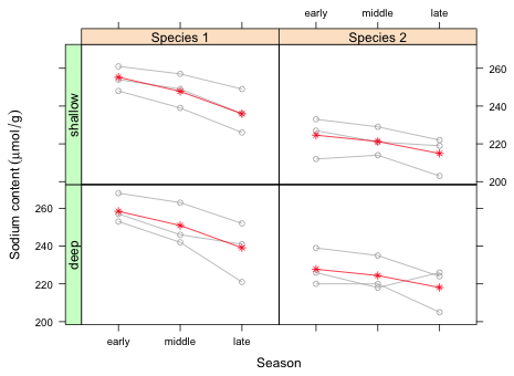
I start by obtaining the population average estimates of the means.
Because season is an ordinal variable I choose to display it on the x-axis. I reset the levels of the season variable so that they're in time order.
Much of the code from lecture 10 can be used here with minimal modification. For the conditioning variables I specify them in the order depth + species so that species varies within a row to facilitate detecting the nature of the species × season interaction. I also improve the labeling of the species variable in the plot and add appropriate labels.
| |
| Fig. 1 Population average mean response ( |
While the interaction between season and species is more or less apparent in Fig. 1, it might be preferable to show both species profiles for a given depth in the same panel. The following code only conditions on depth and plots the profiles for both species in the same panel. It accomplishes this by subsetting the data by species within the panel function.
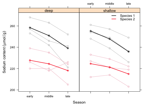 |
| Fig. 2 Population average mean response ( |
I convert the season variable to a numeric variable (the factor levels are coded 1, 2, and 3) and refit the model.
We get the same pattern as before, a significant main effect due to depth and a significant interaction between season and species.
I obtain the predictions from this model and add them to the graph of Fig. 1
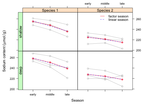 |
| Fig. 3 Comparing the population average mean response for a factor season model and a numeric season model. |
I redo Fig. 2 using the linear model instead of the factor model.
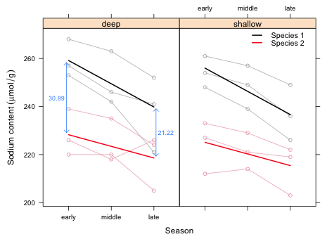 |
| Fig. 4 Population average mean responses (—) and raw data (–o–) for a model in which season is treated as a numeric variable with equally spaced categories. |
From the graph we see that there are two differences between the species.
The summary table of the model is shown below.
The estimated model is
![]()
Because the first numerical value of season is 1 the estimates of the intercept and the species main effect are not directly interpretable in this model. The intercept and the species main effect correspond to when season = 0, a value that is outside the range of the data. Even worse it is unclear what season = 0 could possibly mean given that season actually represents "early", "middle", and "late" , values that we are assuming are equally spaced.
To make the intercept interpretable we should code the numeric season variable so that zero corresponds to the level season = 'early'.
![]()
Now we see that when season = 1 ('early') the sodium content of species 2 eggs is 30.9 units below that of species 1 eggs (the value of β1). During the course of the season the sodium content of species 1 eggs decreases at a rate of 9.67 µmol/g per unit time (β2), but the sodium content of species 2 eggs decreases at a rate of 4.83 µmol/g per unit time, obtained by adding the season effect to the season × species interaction (β2 + β4). (Note: it is entirely fortuitous that the rate for species 2, β2 + β4, and the difference in the rates between species 1 and species 2, β2, are the same.)
When season = 1 ('early') the mean sodium content of the eggs of the two species differs by β1 = 30.89 µmol/g. When season = 3 ('late') the mean sodium content of the eggs differs by only β1 + (3 – 1)β4 = 21.22 µmol/g. We can also calculate this difference by subtracting the prediction of species 2 from species 1 when season = 3.
Table 1 summarizes the estimated differences between the species.
| Table 1 Estimated species effects on egg sodium content |
| Characteristic | Difference: Species 2 – Species 1 |
Species 1 | Species 2 | |
| Rate of change of egg sodium content over time (μmol/g/time) | 4.83 | –9.67 | –4.83 | |
Egg sodium content |
Season = 'early' | –30.89 | varies with depth | |
Season = 'late' |
–21.22 | |||
| Jack Weiss Phone: (919) 962-5930 E-Mail: jack_weiss@unc.edu Address: Curriculum for Ecology and the Environment, Box 3275, University of North Carolina, Chapel Hill, 27599 Copyright © 2012 Last Revised--October 21, 2012 URL: https://sakai.unc.edu/access/content/group/3d1eb92e-7848-4f55-90c3-7c72a54e7e43/public/docs/solutions/assign6.htm |