Lecture 20—Wednesday, October 31, 2012

Topics

• Model selection example—continued
• Model 3: nonlinear Arrhenius model
• Transformed response variables and log-likelihood
  • Transforming the predictor
    • Interpreting log x as a predictor
  • Transforming the response
    • Interpreting log y as a response when x is the predictor
    • Interpreting log y as a response when log x is the predictor
  • Comparing discrete and continuous models using AIC
  • Using AIC to compare a discrete model and a continuous model with a transformed response
• Model 7: Log-transformed response model
• Model 8: Square root transformed response model
• Interpreting the transformed response regression models
• Cited references
• R code

R functions and commands demonstrated

• nls is the nonlinear least squares function for fitting nonlinear models using least squares.

R function options

• start= (argument to nls) specifies the named starting values for parameters in a nonlinear model.

R packages used

• gamlss for separate dispersion negative binomial models.
• MASS for the glm.nb function.

Model selection example—continued

Last time we considered the problem of choosing a statistical model of the species-area relationship. Following Johnson and Raven (1973) and Hamilton et al. (1963) we attempted to find a model relating species richness to area using vascular plant data from the Galapagos islands. I start by refitting the five models we considered last time: normal model in area, normal model in log area, Poisson model in log area, negative binomial model in log area (both NB-2 and NB-1).

Model 3: nonlinear Arrhenius Model

A third normal model we have not yet considered is the Arrhenius model. This model expresses mean species richness as a function of area using the power law equation, and is an example of a nonlinear model. The nls function of R (an acronym for nonlinear least squares) can be used to fit nonlinear models. As part of the model specification the nls function requires initial estimates for the parameters. These get specified by name in the start argument of nls. I choose 0.5 for the initial estimate of b1 because a square root curve appears to be a reasonable guess for the functional relationship seen in a scatter plot of the data. Power functions with exponents between 0 and 1 yield graphs that are concave down while power functions with exponents that are greater than 1 yield graphs that are concave up.

Parameters:
   Estimate Std. Error t value Pr(>|t|)   
b0 33.39760   10.04865   3.324  0.00256 **
b1  0.29857    0.04412   6.767 2.89e-07 ***
---
Signif. codes:  0 ‘***’ 0.001 ‘**’ 0.01 ‘*’ 0.05 ‘.’ 0.1 ‘ ’ 1

Residual standard error: 60.04 on 27 degrees of freedom

Number of iterations to convergence: 10
Achieved convergence tolerance: 3.115e-06

I graph the data and add the estimated Arrhenius model to the scatter plot using the curve function (Fig. 1).

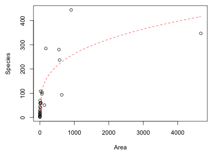
Fig. 1   Nonlinear Arrhenius model

Because of the scale of the plot, the fit is difficult to judge visually. One thing is clear though, the scatter about the fitted curve is not constant; it increases with area. This is something that is not accounted for when a normal distribution is used as the random component of the model. (Recall that in a normal distribution the mean and variance are independent and the variance is constant.) Having said this, notice that the AIC we obtain is the best of the three normal models thus far, but the Arrhenius model does not do as well as the negative binomial models that properly account for the mean-variance relationship.

Transformed response variables and log-likelihood

The two remaining models in our list fit a linear model in log area to a transformed response variable: log species richness or square root species richness. Before considering these two models specifically we need to discuss the use of variable transformations in regression.

Transforming the predictor

We transform a predictor in a regression model in an attempt to obtain a better linear relationship with the response. As we saw last time when we plot species richness against area we fail to see even a hint of linear relationship (Fig. 2a), but when we plot species richness against log(Area) some semblance of a linear relationship does emerge (Fig. 2b). The graph in Fig. 2b as well as the residual plot shown last time suggests that adding an additional quadratic term in log(Area) to the regression equation might still be necessary.

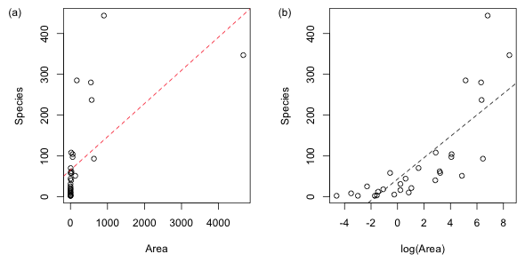Fig. 2  The "linear" relationship between species richness and area (a) before and (b) after applying a log transformation to the predictor.

Interpreting log x as a predictor

Interpreting transformed predictors can be tricky. One way to get a basic understanding of how change in a transformed predictor alters the response is to carry out a linearization. The definition of the derivative tell us

So, if our regression equation is

then the linearization is the following.

The form of the linearization suggests that we ought to consider multiplicative changes in x. Suppose we have a 1% change in x. Then the linearization equation gives us the following.

So a 1% change in x leads to y changing by the amount .01β₁.

Transforming the response

Transformations of a response variable are carried out either to (1) stabilize the variance, i.e., remove variance heterogeneity or (2) achieve normality. In Fig. 2b we see that before and after transforming the predictor there is a good deal of heterogeneity in the spread of the data about the regression line. Two transformations that have been commonly used to stabilize the variance with count data are the log and square root. I try both of these transformations using log(Area) as a predictor and display the results in Fig. 3.

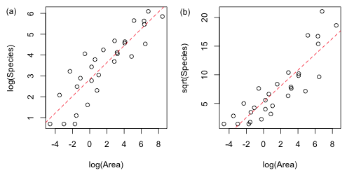Fig. 3  Plot of the two transformed response models (a) log and (b) square root. The displayed regression lines are the means of the transformed response variables.

Both of the transformations shown in Fig. 3 appear to have stabilized the variance, but the plot of log(Species) plotted against log(Area) appears to have also achieved the best linear relationship. Of course there was already a good theoretical basis for using a log transformation on both the response and the predictor. If the theoretical power law relationship for the species-area relationship is correct, then log-transforming both sides of the equation yields a linear equation.

Interpreting log y as the response when x is the predictor

There are two situations to consider, one where y is transformed but x is not and the other where both y and x are transformed. I consider only the case of a log transformation. If we transform y but not x then our regression equation is the following.

If we let z = log y, then the linearization equation tells us

But we can also write

Therefore the approximate change in y is given by the following.

Notice that an absolute change in x leads to a multiplicative effect on y. So a one unit change in x leads to a (100 × β₁)% change in y.

Interpreting log y as the response when log x is the predictor

Finally we consider the case where log y is the response and log x is the predictor. Our regression equation is the following.

To interpret the effect that changing x has on y we just need to combine the previous two results. Let z = log y, then with log x as a predictor we have the following.

Expressing this in terms of Δy yields the following.

Suppose we have a 1% change in x. It then follows that the change in y is the following.

So a 1% change in x leads to a β₁% change in y.

Table 1 summarizes these results for the various possible combinations of response and predictor. In all cases β₁ is the coefficient of the predictor in the regression equation.

Comparing discrete and continuous models using AIC

Three of the six models we've fit so far use a continuous normal distribution for the response and three of the models use a discrete probability model for the response: either a negative binomial or a Poisson distribution. Even though we have both continuous and discrete models we've used AIC to compare them all. This should give you pause. AIC is based on likelihood and the likelihood of a normal model is the product of density functions while the likelihood of a discrete distribution such as the negative binomial model is a product of probabilities.

Densities and probabilities are not directly comparable. To obtain a probability from a density we have to first integrate it over an interval. Furthermore a discrete model like a negative binomial model returns the probability of obtaining a specific count value, e.g., P(Y = 4) whereas the probability of any single value in a continuous probability model is zero. We can only obtain nonzero probabilities with continuous random variables when we consider intervals of the form a < Y < b.

So, when we use a normal distribution to model a discrete random variable such as a count, how are we supposed to interpret the predictions from the model? If our goal is to calculate P(Y = 4) then a sensible approach is to treat all values of Y that round to 4 as corresponding to the discrete value 4. Hence, we should define P(Y = 4) = P(3.5 < Y ≤ 4.5). For a normal regression model this is the area under the normal curve between Y = 3.5 and Y = 4.5 (Fig. 4a).

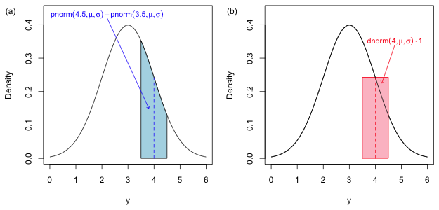Fig. 4  The probability of a discrete count, P(Y = 4), when we use a continuous model is defined to be the probability of the set of values that round to 4, P(3.5 < Y ≤ 4.5). (a) shows the exact probability of this quantity while (b) shows how this probability can be approximated as the area of a rectangle obtained using the midpoint rule for numerical integration.

When the notion of the integral is first developed in a calculus class as the area under a curve, one typically starts by trying to approximate that area using methods based on summing the areas of approximating rectangles. One such method is the midpoint rule. To approximate the area shown in Fig. 4a we evaluate the function at the midpoint of the interval (3.5, 4.5) and use that value as the height of a rectangle. We then multiply the height by the width of the interval to obtain an approximation of the area under the curve.

Thus the density function evaluated at discrete values also approximates the probability of that discrete value. So, when we use a continuous probability model for a discrete random variable the densities that occur in the likelihood are each approximations (Fig. 4b) of the exact probabilities (Fig. 4a). Typically the exact probabilities and the approximations based on the midpoint rule are quite close. For instance, for the normal distribution shown in Fig. 4 where μ = 3 and σ =1 we find the following.

So, we have accuracy to three decimal places. Thus it is legitimate to compare the AICs of discrete models and continuous models when the continuous models are being used to approximate a discrete random variable whose domain is the set of non-negative integers.

Using AIC to compare a discrete model and a continuous model with a transformed response

In lecture 19 we listed some caveats associated with using AIC to compare different models. Caveat 2 noted that the response variable must be the same in all models being compared. Thus if we log-transform a response and assume that the transformed variable has a normal distribution, the likelihood of the transformed variable model is not comparable to the likelihood of a probability model with an untransformed response. Returning to the Galapagos data set suppose we log-transform the response and assume that the transformed response has a normal distribution. We fit that model below and calculate its AIC.

The lowest AIC we've previously obtained has been 273.99 with the negative binomial (NB-2) model. The reported AIC of the lognormal model is lower than that this but according to caveat 2 we should draw no conclusion from this because the likelihoods of the two models are not comparable. Fig. 5 illustrates the basic problem.

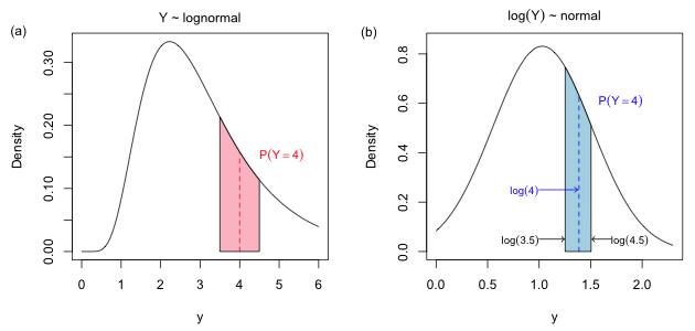Fig. 5  The figure shows the area that corresponds to the discrete probability, P(Y = 4). In Fig. 4a the probability is the area under the lognormal curve P(3.5 < Y < 4.5). In Fig. 4b it is the area under the normal curve P(log 3.5 < Z < log 4.5) where Z = log Y. If we approximate these area using the midpoint rule the width of the approximating rectangle in Fig. 4a is 1, but the width of the same rectangle in Fig. 4b is log 4.5 – log 3.5.

When the log-transformed version of a variable has a normal distribution, we say that the original variable has a lognormal distribution. The R density function for the lognormal distribution is dlnorm. Following the same logic that we used in Fig. 3 we would calculate P(Y = 4) as P(3.5 < Y ≤ 4.5). This is shown in Fig. 5a.

So we can construct a likelihood for a discrete random variable using the continuous lognormal densities and treat the product of densities as an approximation to the probability of our data. Here I use μ* and σ* to denote the two parameters of the lognormal distribution. In the usual parameterization of the lognormal distribution μ* is the mean of log(Y) and σ* is the standard deviation of log(Y).

But this is not the same as the likelihood that we would construct from the log-transformed response. From Fig. 5b we would calculate P(Y = 4) as follows.

because log 4.5 – log 3.5 ≠ 1. So the density of the log-transformed predictor is not an approximation of P(Y = 4). We can salvage things but it involves constructing the log-likelihood ourselves. There are two options.

1. Use the midpoint rule for each y but rescale the normal density, dnorm(log 4, μ, σ), so that it correctly approximates the area under the curve. The rescaling constant turns out to be the derivative of the transformation.
2. For each y calculate the exact area under the curve using the difference of cumulative distributions: pnorm(log (4.5), μ, σ) – pnorm(log (3.5), μ, σ).

If the response variable y is continuous then we should use (1) because we are comparing densities, not probabilities. If the response variable y is discrete then we should use (2). In truth when y is discrete both options will work except when there are zero values of y in the data set. In that case using the midpoint rule to calculate probabilities can yield wildly inaccurate estimates.

Model 7: Log-transformed response model

If Y is a discrete non-negative random variable with no zero values then log Y is well-defined. In that case as discussed above P(Y_i = y_i) can be calculated as follows.

The likelihood is therefore the following.

Y = 0 is a boundary value so for zero values of Y we have to define P(Y = 0) = P(Y ≤ 0.5). Because log Y is undefined for Y = 0, the usual recommendation when there are zero values of Y is to add a small constant c to each of the data values before taking the log. Choices of c = 1 or c = 0.5 are common. In this case the likelihood will consist of two distinct terms depending upon whether Y = 0 or not.

The R function shown below implements this formula for a normal model with a log-transformed response variable. It takes as input arguments the raw response variable (before being transformed) and the name of the model. It has an optional argument c set by default to zero that can be specified if a constant has been added to the response to adjust for zero values. The first line of the function estimates σ² by squaring the residuals of the model and dividing by how many observations there are. This is the MLE of σ² and is different from the usual estimate returned by lm. The return values of the function are the log-likeihood, the number of model parameters, and the AIC.

I try it out on a log-transformed response model with log(Area) as the regressor.

Comparing this result to the models we've fit so far we see that this model ranks second after the negative binomial NB-2 model. The difference in AIC between it and the NB-2 model is quite small.

Model 8: Square root transformed response model

A similar approach works with the square root transformation. We calculate the log-likelihood in the same way replacing the log transformation with the square root function. Even though there is really no need for it I keep the option of adding a small constant to the response because the literature has sometimes recommended adding a constant before taking the square root.

I assemble the model results in a single table where I also include the log-likelihoods of the models fit thus far.

Finally I sort the models by their AIC values.

Based on the output we see there are only two models that have substantial empirical support, the Arrhenius model (out.lognormal) and the negative binomial model (out.NB2), both of which use log(Area) as the predictor. Other than the NB-1 model none of the other models are even players. While the negative binomial model just edges out the Arrhenius model, these two models are virtually identical in terms of log-likelihood and AIC. So using these criteria alone there is little basis for choosing one over the other. Both of these models allow for heteroscedasticity in the data and the assumed form of the heteroscedasticity is roughly the same for each. As will be explained in the next section there is a practical reason to perhaps prefer the negative binomial. The negative binomial model estimates the mean richness while the Arrhenius model estimates the median richness when we back-transform to the raw richness scale.

Interpreting the transformed response regression models

Can we interpret a regression model for the transformed response variable on the scale of the raw response variable? Yes, but the prediction we obtain is not the mean. The three count models we've fit, models 4, 5 and 6, use a log link function and thus fit a model for log μ.

models 4, 5 and 6:

With a log link recovering the mean is easy; we just exponentiate both sides of this equation to remove the logarithm.

With a log-transformed response (and an identity link) we fit a regression model to the mean of the transformed response variable.

model 7:

The logarithm function now is shielded by the mean function. We can still exponentiate both sides but unlike the case with a log link the result will not be the mean. The logarithm is an example of a concave function. A concave function is one that lies above any secant line drawn connecting two points on its curve. For a concave function f a relationship called Jensen's inequality tells us that

For the logarithm function Jensen's inequality states that the log of a mean of a set of values exceeds the mean of log of those same values. Fig. 6 demonstrates Jensen's equality for f(x) = log x where the data set consists of just the two numbers {1, 3}. The mean of these two numbers is 2. I plot on the graph the log of their mean, log 2, as well as the mean of their logs: (log 1 + log 3) /2. The mean of the logs lies on the line segment connecting (1, log 1) to (3, log 3) while log of the mean lies on logarithm curve. As Fig. 6 shows the log of the mean exceeds the mean of the logs.

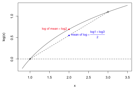
Fig. 6   An illustration of Jensen's inequality for concave functions: log μ(x) ≥ μ(log x)

In fitting the model out.lognormal we assumed that the log-transformed richness variable had a normal distribution. By definition, if a log-transformed random variable has a normal distribution, then the original response variable is said to have a lognormal distribution. While the mode, median, and mean of a normal distribution are all the same, in a lognormal distribution the mode, median, and mean are typically different.

The exponential function is a monotone function because . As a result if we exponentiate both sides of the log-transformed regression equation of model 7 the relative order of the values will not change. Quantiles on the log-transformed scale will get mapped to quantiles on the raw response scale. In particular the median on the log-transformed scale will get mapped to the median on the raw scale. So when we exponentiate the regression equation of model 7 (which is a model for the mean log, but also the median and mode of log S) we do get the median richness of a lognormal distribution on the original raw scale. The mean and mode on the other hand are not the same. Fig. 7 shows the relationships between these statistics for the sixth island, Daphne Major, whose predicted log species richness is 1.62.

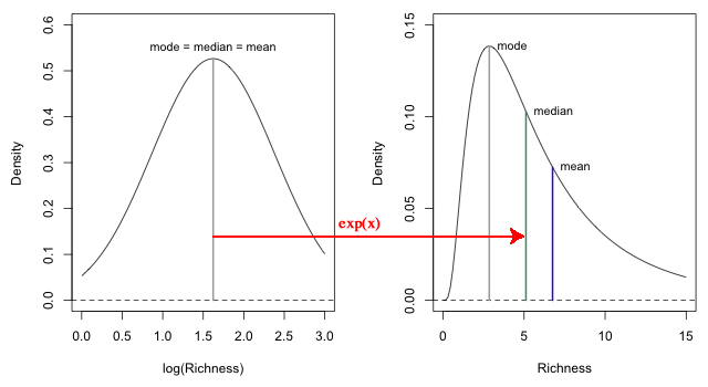Fig. 7  When the regression equation of a log-transformed response is back-transformed by exponentiating both sides, we obtain a regression equation for the median on the scale of the original response variable, not the mean.

A lognormal distribution is typically positively skewed so that the median and mean can be very different. The mean μ* of the lognormal distribution can be expressed in terms of μ and σ², the mean and variance of the log-transformed variables.

This makes it possible to calculate the mean raw response after fitting a regression model to the log-transformed response. Because the square root transformation is also a monotonic transformation, squaring its regression equation will also yield a regression equation for the median on the original richness scale.

Fig. 8 graphically compares the four AIC-best ranked models for the Galapagos flora data set. It shows both predicted mean and the predicted median of the lognormal distribution corresponding to the log-transformed response normal model.

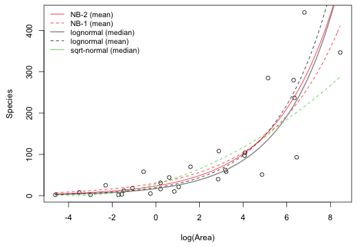Fig. 8    Fitted regression equations for the four AIC-best models. Shown are the two negative binomial means (NB-1 and NB-2), the lognormal mean and lognormal median, and the square root normal median.

Cited References

• Hamilton, Terrell H., Ira Rubinoff, Robert H. Barth, Jr., and Guy L. Bush. 1963. Species abundance: natural regulation of insular variation. Science 142: 1575–1576.
• Johnson, Michael P. and Peter H. Raven. 1973. Species number and endemism: The Galapagos archipelago revisited. Science 179: 893–895.

R Code

A compact collection of all the R code displayed in this document appears here.

Course Home Page