We see that the SlopeAspect variable has a lot of missing data.
In order to fit a classification tree we have to convert the response variable, Occupied_Unoccupied, into a factor.
node), split, n, loss, yval, (yprob)
* denotes terminal node
1) root 454 207 0 (0.5440529 0.4559471)
2) TotalCanopy< 8.2 210 40 0 (0.8095238 0.1904762)
4) WildIndigoSize< 58.88 127 9 0 (0.9291339 0.0708661) *
5) WildIndigoSize>=58.88 83 31 0 (0.6265060 0.3734940)
10) DistanceNearestTree>=595 46 5 0 (0.8913043 0.1086957) *
11) DistanceNearestTree< 595 37 11 1 (0.2972973 0.7027027)
22) DirectionTree>=247.5 9 4 0 (0.5555556 0.4444444) *
23) DirectionTree< 247.5 28 6 1 (0.2142857 0.7857143) *
3) TotalCanopy>=8.2 244 77 1 (0.3155738 0.6844262)
6) WildIndigoSize< 58.155 116 49 0 (0.5775862 0.4224138)
12) TotalCanopy>=65.235 33 2 0 (0.9393939 0.0606061) *
13) TotalCanopy< 65.235 83 36 1 (0.4337349 0.5662651)
26) TotalCanopy< 18.88 30 5 0 (0.8333333 0.1666667) *
27) TotalCanopy>=18.88 53 11 1 (0.2075472 0.7924528) *
7) WildIndigoSize>=58.155 128 10 1 (0.0781250 0.9218750) *
|
|---|
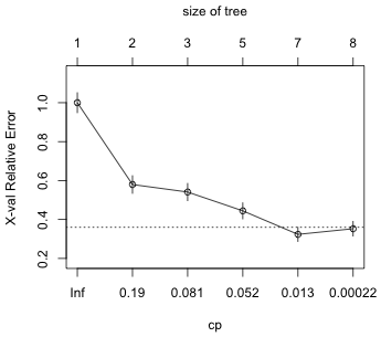
| Fig. 1 Plot of cross-validation error versus Cp |
The plot is unambiguous. The first tree whose cross-validation error is within one standard deviation of the minimum cross-validation error is the tree with minimum cross-validation error. We should select a tree of size 7 (nsplit = 6) corresponding to Cp = 0.0048.
 |
|---|
| Fig. 2 Pruned classification tree |
I fit a GAM using all the predictors and then try to simplify it. We can't specify more knots than there are unique values (the default choice is k = 10), so I determine the number of unique values for each variable.
We need to use no more than 8 knots for DirectionTree and SlopeAspect.
Formula:
Occupied_Unoccupied ~ s(TotalCanopy) + s(WildIndigoSize) + s(NearestWildIndigo) +
s(DistanceNearestTree) + s(DirectionTree, k = 8) + s(Slope) +
s(SlopeAspect, k = 8)
Parametric coefficients:
Estimate Std. Error z value Pr(>|z|)
(Intercept) -0.6010 0.3566 -1.685 0.0919 .
---
Signif. codes: 0 ‘***’ 0.001 ‘**’ 0.01 ‘*’ 0.05 ‘.’ 0.1 ‘ ’ 1
Approximate significance of smooth terms:
edf Ref.df Chi.sq p-value
s(TotalCanopy) 3.409 4.249 31.697 2.96e-06 ***
s(WildIndigoSize) 1.000 1.000 32.884 9.79e-09 ***
s(NearestWildIndigo) 1.000 1.000 9.586 0.00196 **
s(DistanceNearestTree) 2.091 2.629 4.592 0.16224
s(DirectionTree) 1.000 1.000 3.928 0.04749 *
s(Slope) 1.000 1.000 0.054 0.81608
s(SlopeAspect) 1.000 1.000 0.667 0.41416
---
Signif. codes: 0 ‘***’ 0.001 ‘**’ 0.01 ‘*’ 0.05 ‘.’ 0.1 ‘ ’ 1
R-sq.(adj) = 0.58 Deviance explained = 53.1%
ML score = 116.83 Scale est. = 1 n = 328
The summary table suggests that Slope and SlopeAspect are not significant, but we know that the p-values of the Wald tests for GAMs can be quite unreliable. The different reduced models we might fit and compare against this one are not all equivalent because the variable SlopeAspect has a large number of missing values.
The gam function will silently remove these missing values anytime SlopeAspect is a predictor in the model. Models that are fit to different sets of observations cannot be compared using significance testing or AIC. It makes sense to test SlopeAspect first because if it can be dropped then the remaining variables can be examined using the full data set. To make models with and without SlopeAspect comparable I need to explicitly remove the observations that have missing values for SlopeAspect before fitting the model without SlopeAspect.
As was explained in lecture 39, the default number of knots (10) is set too low for a number of these smooths and has the effect of constraining then. As a result, when SlopeAspect is removed from the model it partially releases this constraint causing the two models to use different smoothing parameters. These models are then not truly nested and the likelihood ratio test is invalid. We can fix this by increasing the number of knots and/or using the smoothing parameters from the bigger model in the smaller model.
Model 1: Occupied_Unoccupied ~ s(TotalCanopy, k = 20) + s(WildIndigoSize,
k = 20) + s(NearestWildIndigo, k = 20) + s(DistanceNearestTree,
k = 20) + s(DirectionTree, k = 8) + s(Slope)
Model 2: Occupied_Unoccupied ~ s(TotalCanopy, k = 20) + s(WildIndigoSize,
k = 20) + s(NearestWildIndigo, k = 20) + s(DistanceNearestTree,
k = 20) + s(DirectionTree, k = 8) + s(Slope) + s(SlopeAspect,
k = 8)
Resid. Df Resid. Dev Df Deviance
1 317.41 213.32
2 316.42 212.53 0.9898 0.79907
We can drop SlopeAspect. With that taken care of I refit the model to the full data set.
Family: binomial
Link function: logit
Formula:
Occupied_Unoccupied ~ s(TotalCanopy, k = 20) + s(WildIndigoSize,
k = 20) + s(NearestWildIndigo, k = 20) + s(DistanceNearestTree,
k = 20) + s(DirectionTree, k = 8) + s(Slope)
Parametric coefficients:
Estimate Std. Error z value Pr(>|z|)
(Intercept) -0.7841 0.2947 -2.66 0.0078 **
---
Signif. codes: 0 ‘***’ 0.001 ‘**’ 0.01 ‘*’ 0.05 ‘.’ 0.1 ‘ ’ 1
Approximate significance of smooth terms:
edf Ref.df Chi.sq p-value
s(TotalCanopy) 3.514 4.408 37.816 2.04e-07 ***
s(WildIndigoSize) 2.532 3.172 52.407 3.24e-11 ***
s(NearestWildIndigo) 1.000 1.000 13.037 0.000305 ***
s(DistanceNearestTree) 3.281 4.091 8.895 0.067595 .
s(DirectionTree) 1.000 1.000 4.152 0.041576 *
s(Slope) 1.000 1.000 0.179 0.672329
---
Signif. codes: 0 ‘***’ 0.001 ‘**’ 0.01 ‘*’ 0.05 ‘.’ 0.1 ‘ ’ 1
R-sq.(adj) = 0.587 Deviance explained = 53.1%
ML score = 164.05 Scale est. = 1 n = 454
Slope is the next candidate to be dropped. I use the same smoothing parameters
Model 1: Occupied_Unoccupied ~ s(TotalCanopy, k = 20) + s(WildIndigoSize,
k = 20) + s(NearestWildIndigo, k = 20) + s(DistanceNearestTree,
k = 20) + s(DirectionTree, k = 8)
Model 2: Occupied_Unoccupied ~ s(TotalCanopy, k = 20) + s(WildIndigoSize,
k = 20) + s(NearestWildIndigo, k = 20) + s(DistanceNearestTree,
k = 20) + s(DirectionTree, k = 8) + s(Slope)
Resid. Df Resid. Dev Df Deviance Pr(>Chi)
1 441.66 293.59
2 440.67 293.43 0.98928 0.15979 0.685
Slope can be dropped. I refit the model using its own smoothing parameters.
Formula:
Occupied_Unoccupied ~ s(TotalCanopy, k = 20) + s(WildIndigoSize,
k = 20) + s(NearestWildIndigo, k = 20) + s(DistanceNearestTree,
k = 20) + s(DirectionTree, k = 8)
Parametric coefficients:
Estimate Std. Error z value Pr(>|z|)
(Intercept) -0.7793 0.2893 -2.694 0.00707 **
---
Signif. codes: 0 ‘***’ 0.001 ‘**’ 0.01 ‘*’ 0.05 ‘.’ 0.1 ‘ ’ 1
Approximate significance of smooth terms:
edf Ref.df Chi.sq p-value
s(TotalCanopy) 3.527 4.420 37.900 1.99e-07 ***
s(WildIndigoSize) 2.629 3.294 52.377 3.99e-11 ***
s(NearestWildIndigo) 1.000 1.000 13.167 0.000285 ***
s(DistanceNearestTree) 3.238 4.036 8.795 0.067999 .
s(DirectionTree) 1.000 1.000 4.132 0.042079 *
---
Signif. codes: 0 ‘***’ 0.001 ‘**’ 0.01 ‘*’ 0.05 ‘.’ 0.1 ‘ ’ 1
R-sq.(adj) = 0.588 Deviance explained = 53.1%
ML score = 164.14 Scale est. = 1 n = 454
DistanceNearestTree is the next candidate to be dropped. I consider a likelihood ratio test.
Model 1: Occupied_Unoccupied ~ s(TotalCanopy, k = 20) + s(WildIndigoSize,
k = 20) + s(NearestWildIndigo, k = 20) + s(DirectionTree,
k = 8)
Model 2: Occupied_Unoccupied ~ s(TotalCanopy, k = 20) + s(WildIndigoSize,
k = 20) + s(NearestWildIndigo, k = 20) + s(DistanceNearestTree,
k = 20) + s(DirectionTree, k = 8)
Resid. Df Resid. Dev Df Deviance Pr(>Chi)
1 443.64 315.02
2 441.61 293.41 2.0304 21.607 2.129e-05 ***
---
Signif. codes: 0 ‘***’ 0.001 ‘**’ 0.01 ‘*’ 0.05 ‘.’ 0.1 ‘ ’ 1
The likelihood ratio test and Wald test are in strong disagreement. The likelihood ratio test argues we should retain DistanceNearestTree. So our final model has the smooths of five predictors of which three appear to be nonlinear (based on the reported edf) and two are linear.
My basic strategy is to fit a logistic regression model using all of the variables and then gradually weed out those predictors that are flawed and/or have no relationship to the responses. I use the tree results as well as a GAM to suggest interactions and improve the structural forms for the various remaining predictors. I start the process by including all the variables individually and additively in a logistic regression model
Dealing with the angle variables
The variable SlopeAspect is an obvious candidate for omission. Recall that SlopeAspect is a variable with a lot of missing values. Both Slope and SlopeAspect are angles and angles require some care when including them in regression models. I examine their values.
The values for Slope are all rather close so nothing more needs to be done with it, but SlopeAspect has a wide range. Angles are circular measures and consequently 0 and 360 are the same angle. This means on a circular scale that 315 is as close to 0 as 45 is to 0. Currently in the regression model 0 and 315 are treated as being the the furthest apart. How angle should be included in a regression model depends on how we think angle impacts the response. This is a substantive issue not a statistical one. Having said that it is almost certainly the case given the range of the data that using the raw angle measured in degrees makes very little sense. One possibility is to use the cosine or sine of the angles. I try each in turn and both together.
The model with lowest AIC uses cosine. If we examine the summary table we find that its coefficient is not significant. So, we can drop it.
Slope is not significant so I drop it next.
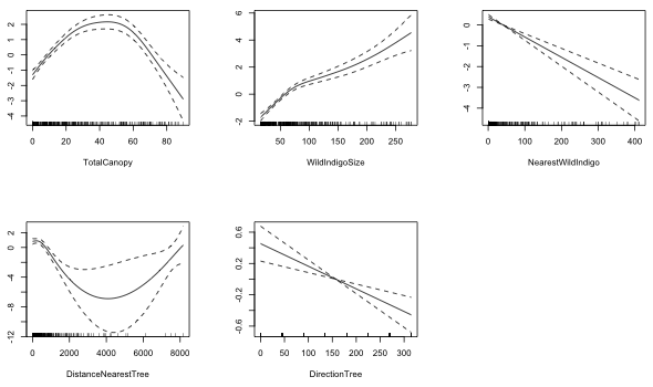
At this point all the terms remaining in the model were also in our final GAM model. I examine the graphs of their smooths.
 |
|---|
Fig. 3 Plots of the estimated smooths from a generalized additive model (GAM) |
NearestWildIndigo and DirectionTree look linear. DirectionTree has some other issues that we'll deal with later. The remaining variables look nonlinear. The smooth for TotalCanopy looks very much like a quadratic function. I try that next.
The quadratic term is significant. The relationship with DistanceNearestTree also looks quadratic. I try that next.
The quadratic term is again significant. The partial response function for WidIndigoSize looks like a logarithm. I replace WildIndigoSize with log(WildIndigoSize) and then compare these two models using AIC.
So the log model is preferred. The summary table of our model thus far is shown below.
DirectionTree is a weird variable. Does it make sense to treat it as continuous? Currently the coefficient is negative and significant. So that means as the angle to the next tree gets bigger, we're less likely to find the butterfly. If we examine the variable we see that it has only a few unique values.
I try taking the sine and cosine of the angle as well as treating it as a factor.
So, the linear model ranks best although the factor model comes close. The likelihood ratio tests for for both are statistically significant.
Model 1: Occupied_Unoccupied ~ TotalCanopy + NearestWildIndigo + DistanceNearestTree +
I(TotalCanopy^2) + I(DistanceNearestTree^2) + log(WildIndigoSize)
Model 2: Occupied_Unoccupied ~ TotalCanopy + NearestWildIndigo + DistanceNearestTree +
I(TotalCanopy^2) + I(DistanceNearestTree^2) + log(WildIndigoSize) +
factor(DirectionTree)
Resid. Df Resid. Dev Df Deviance Pr(>Chi)
1 447 312.65
2 440 297.09 7 15.558 0.02948 *
---
Signif. codes: 0 ‘***’ 0.001 ‘**’ 0.01 ‘*’ 0.05 ‘.’ 0.1 ‘ ’ 1
Model 1: Occupied_Unoccupied ~ TotalCanopy + NearestWildIndigo + DistanceNearestTree +
I(TotalCanopy^2) + I(DistanceNearestTree^2) + log(WildIndigoSize)
Model 2: Occupied_Unoccupied ~ TotalCanopy + NearestWildIndigo + DistanceNearestTree +
DirectionTree + I(TotalCanopy^2) + I(DistanceNearestTree^2) +
log(WildIndigoSize)
Resid. Df Resid. Dev Df Deviance Pr(>Chi)
1 447 312.65
2 446 308.36 1 4.2947 0.03823 *
---
Signif. codes: 0 ‘***’ 0.001 ‘**’ 0.01 ‘*’ 0.05 ‘.’ 0.1 ‘ ’ 1
As a final comparison I plot the partial response functions for the factor model and the linear model for DirectionTree and superimpose them. To simplify obtaining the factor model estimates I refit the model without the intercept.
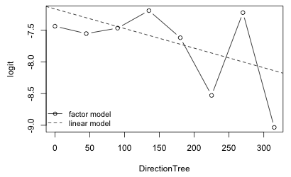 |
|---|
Fig. 3 Fitted relationship between logit and DirectionTree variable: individual estimates for each angle from a factor model as well as the estimated linear relationship. |
It's difficult to tell if DirectionTree is capturing anything real in the data. The means for individual angles show an extreme amount of variability about the regression line.
Because TotalCanopy appears repeatedly on the right branch of the classification tree, it suggests that the response may have a nonlinear relationship with TotalCanopy. The GAM has already suggested a quadratic relationship so we don't learn anything more about nonlinearities from looking at the classification tree.
The variables TotalCanopy, WildIndigoSize, and DistanceNearestTree occur along a single branch of the classification tree. This may indicate that in an ordinary logistic regression model including interactions between TotalCanopy, WildIndigoSize, and DistanceNearestTree might be a good choice. On the other hand the right branch also includes TotalCanopy and WildIndigoSize with nearly the same split value for WildIndigoSize. So perhaps only one of the component two-factor interactions is required. I try adding an interaction between these three variables. Each of the variables has a modified form in the model, two of them are quadratic and one is logged, so choosing the proper form for the interaction is complicated. For instance we could choose to involve the quadratic terms.
Model 1: Occupied_Unoccupied ~ TotalCanopy + NearestWildIndigo + DistanceNearestTree +
DirectionTree + I(TotalCanopy^2) + I(DistanceNearestTree^2) +
log(WildIndigoSize)
Model 2: Occupied_Unoccupied ~ TotalCanopy + NearestWildIndigo + DistanceNearestTree +
DirectionTree + I(TotalCanopy^2) + I(DistanceNearestTree^2) +
log(WildIndigoSize) + TotalCanopy:log(WildIndigoSize) + TotalCanopy:DistanceNearestTree +
DistanceNearestTree:log(WildIndigoSize) + TotalCanopy:DistanceNearestTree:log(WildIndigoSize)
Resid. Df Resid. Dev Df Deviance Pr(>Chi)
1 446 308.36
2 442 301.11 4 7.2454 0.1235
Model: binomial, link: logit
Response: Occupied_Unoccupied
Terms added sequentially (first to last)
Df Deviance Resid. Df Resid. Dev Pr(>Chi)
NULL 453 625.85
TotalCanopy 1 21.830 452 604.02 2.979e-06 ***
NearestWildIndigo 1 55.862 451 548.16 7.772e-14 ***
DistanceNearestTree 1 65.682 450 482.47 5.298e-16 ***
DirectionTree 1 3.590 449 478.88 0.058122 .
I(TotalCanopy^2) 1 87.980 448 390.90 < 2.2e-16 ***
I(DistanceNearestTree^2) 1 10.481 447 380.42 0.001206 **
log(WildIndigoSize) 1 72.069 446 308.35 < 2.2e-16 ***
TotalCanopy:log(WildIndigoSize) 1 0.951 445 307.40 0.329508
TotalCanopy:DistanceNearestTree 1 1.100 444 306.30 0.294269
DistanceNearestTree:log(WildIndigoSize) 1 0.157 443 306.15 0.691767
TotalCanopy:DistanceNearestTree:log(WildIndigoSize) 1 5.037 442 301.11 0.024805 *
---
Signif. codes: 0 ‘***’ 0.001 ‘**’ 0.01 ‘*’ 0.05 ‘.’ 0.1 ‘ ’ 1
The three-factor interaction by itself is significant (p= 0.024). The principle of marginality requires that if we add a three-factor interaction to model then we must also add all the component two-factor interactions and main effects. If we carry out a likelihood ratio test of all the interactions simultaneously the test statistic is not significant (p = 0.125). In addition the AIC is higher for the three-factor interaction model (325.1 versus 324.3).
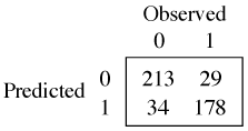
The predict function applied to a classification tree yields the predicted probabilities of each response category separately for each observation.
In each row of the output from predict the entry with the larger probability is the prediction for that observation. Because the values sum to 1 in each row, the prediction is the entry whose value exceeds 0.5.
We could also have obtained this by using the type='class' argument of predict.
I calculate the fraction of correct predictions.
88.3% of the observations are classified correctly as true positives and true negatives.
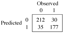
GAM
For the GAM I use model gam3 with five smooths.
s(TotalCanopy) + s(WildIndigoSize) + s(DistanceNearestTree) + s(NearestWildIndigo) + s(DirectionTree)
86.1% of the observations are classified correctly as true positives and true negatives.
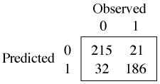
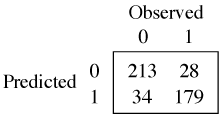
For the logistic regression model I use model mod5.
Occupied_Unoccupied ~ TotalCanopy + NearestWildIndigo + DistanceNearestTree + DirectionTree + I(TotalCanopy^2) + I(DistanceNearestTree^2) + log(WildIndigoSize)
[1] 0.8568282
85.7% of the observations are classified correctly as true positives and true negatives.
| Classification tree | Generalized additive model |
|---|---|
 |
 |
| Logistic regression |
Logistic regression (with interactions) |
 |
 |
Both the classification tree and GAM models beat the logistic regression model in having both fewer false positive and false negatives. The classification tree has individually the fewest number of false positives and false negatives of the three models.
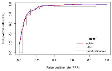
I display the ROC curves for the logistic model, the GAM, and the classification tree. As we saw in Question 3, applying the predict function to a classification tree yields the probability of 0 (column 1) and the probability of 1 (column 2). For the ROC curve we need the probability of 1.
 |
|---|
Fig. 5 ROC curves for a logistic regression model, a five-variable GAM, and a classification tree. |
All of these values are exceedingly high.
Because the classification tree has only six splits, its ROC curve has six jumps. Because the logistic regression model and the GAM treat the variables as continuous, their ROC curves are much smoother. As a result the AUC for these models exceed that of the classification tree. Thus for certain cut-points (0.5 for instance) the classification tree beats both logistic regression models (although rarely the GAM) but on average it does worse. So surprisingly the parametric and semi-parametric models beat the algorithmic approach here. The GAM is the clear winner but does so perhaps by sacrificing interpretability and overfitting the data. In truth all four models do a spectacular job of classification here.
| Jack Weiss Phone: (919) 962-5930 E-Mail: jack_weiss@unc.edu Address: Curriculum for the Environment and Ecology, Box 3275, University of North Carolina, Chapel Hill, 27599 Copyright © 2012 Last Revised--May 2, 2012 URL: https://sakai.unc.edu/access/content/group/2842013b-58f5-4453-aa8d-3e01bacbfc3d/public/Ecol562_Spring2012/docs/solutions/finalpart2.htm |