These are binomial data where we are given the number of successes (dead) out of a total (n). To fit this model in R the response variable needs to be a matrix in which the first column is the number of successes and the second column is the number of failures. Hence we use cbind(dead, n-dead) as the response. To address the question, "Does the dose-response relationship vary by product?" we need to fit a model in which logdose and product interact.
Model: binomial, link: logit
Response: cbind(dead, n - dead)
Terms added sequentially (first to last)
Df Deviance Resid. Df Resid. Dev Pr(>Chi)
NULL 50 311.241
logdose 1 238.854 49 72.387 < 2.2e-16 ***
product 2 0.206 47 72.181 0.9022
logdose:product 2 29.876 45 42.305 3.255e-07 ***
---
Signif. codes: 0 ‘***’ 0.001 ‘**’ 0.01 ‘*’ 0.05 ‘.’ 0.1 ‘ ’ 1
The analysis of deviance table reveals a statistically significant interaction between log dose and product. So we conclude that the dose-response relationship varies by product.
To determine if the residual deviance is suitable here as a goodness of fit statistic we need to examine the expected counts. If no more than 20% of the expected counts are less than 5, the chi-squared distribution of the deviance is reasonable. I use the fitted function to obtain the estimated probabilities and use them to calculate the expected number of successes and failures.
So 24.5% of the counts are less than 5. The use of the residual deviance as as a goodness of fit statistic is suspect here.
To determine if the model can be simplified I examine the summary table for the model.
Deviance Residuals:
Min 1Q Median 3Q Max
-2.39800 -0.60734 0.09695 0.65920 1.69300
Coefficients:
Estimate Std. Error z value Pr(>|z|)
(Intercept) -2.0410 0.3034 -6.728 1.72e-11 ***
logdose 2.8768 0.3432 8.383 < 2e-16 ***
productB 1.2920 0.3845 3.360 0.00078 ***
productC -0.3079 0.4308 -0.715 0.47469
logdose:productB -1.6457 0.4220 -3.899 9.65e-05 ***
logdose:productC 0.4318 0.4898 0.882 0.37793
---
Signif. codes: 0 ‘***’ 0.001 ‘**’ 0.01 ‘*’ 0.05 ‘.’ 0.1 ‘ ’ 1
(Dispersion parameter for binomial family taken to be 1)
Null deviance: 311.241 on 50 degrees of freedom
Residual deviance: 42.305 on 45 degrees of freedom
AIC: 201.31
Number of Fisher Scoring iterations: 4
From the output we see that the dose response relationship for product C is not different than it is for product A , the reference group (p = .038). On the other hand the dose-response relationship of products A and B are clearly different (p < .001). This suggests we might collapse products A and C together and refit the model.
There are two new models we can fit. We can force products A and C to have the same slopes (on a logit scale) but different intercepts. If this model holds, the dose effect is the same but one of the products consistently kills more bugs than the other. We can also force them to have both the same slopes and intercepts so that the products are not different at all.
The three-product model fits the following regression model.
To see if A and C should have the same slopes (same dose-response relationship) we carry out the test
H0: β5 = 0
H1: β5 ≠ 0
I compare out2 with out1 with a likelihood ratio test.
Model 1: cbind(dead, n - dead) ~ logdose + product + logdose:newprod
Model 2: cbind(dead, n - dead) ~ logdose * product
Resid. Df Resid. Dev Df Deviance Pr(>Chi)
1 46 43.083
2 45 42.305 1 0.77817 0.3777
The models are not significantly different so we can use the simpler model in which the slopes of A and C are the same. Said differently we fail to reject that β5 = 0. Hence we don't need to include this term in the model. Our model is now the following.
![]()
I next test whether the intercepts are also the same (meaning that the two products are identical). Formally we carry out the following hypothesis test.
H0: β3 = 0
H1: β3 ≠ 0
Model 1: cbind(dead, n - dead) ~ logdose * newprod
Model 2: cbind(dead, n - dead) ~ logdose + product + logdose:newprod
Resid. Df Resid. Dev Df Deviance Pr(>Chi)
1 47 43.111
2 46 43.083 1 0.0273 0.8688
So we fail to reject the null hypothesis. Therefore the intercepts of A and C are not different. We conclude that products A and C are not different in their killing power.
Deviance Residuals:
Min 1Q Median 3Q Max
-2.2507 -0.6634 0.1382 0.7080 1.6930
Coefficients:
Estimate Std. Error z value Pr(>|z|)
(Intercept) -2.1997 0.2152 -10.223 < 2e-16 ***
logdose 3.0988 0.2444 12.679 < 2e-16 ***
newprodB 1.4507 0.3196 4.539 5.64e-06 ***
logdose:newprodB -1.8677 0.3465 -5.390 7.06e-08 ***
---
Signif. codes: 0 ‘***’ 0.001 ‘**’ 0.01 ‘*’ 0.05 ‘.’ 0.1 ‘ ’ 1
(Dispersion parameter for binomial family taken to be 1)
Null deviance: 311.241 on 50 degrees of freedom
Residual deviance: 43.111 on 47 degrees of freedom
AIC: 198.11
Number of Fisher Scoring iterations: 4
From the summary table of the final model we see that product B has a significantly lower slope than do products A and C together.
Alternatively we could jump over the intermediate model and test whether we need do distinguish product C from product A at all.
H0: β3 = β5 = 0
H1: at least one of β3 and β5 are not zero
We carry out analysis of deviance on out1 and out3.
Model 1: cbind(dead, n - dead) ~ logdose * newprod
Model 2: cbind(dead, n - dead) ~ logdose * product
Resid. Df Resid. Dev Df Deviance Pr(>Chi)
1 47 43.111
2 45 42.305 2 0.80547 0.6685
So we fail to reject the null hypothesis and conclude that we do not need to distinguish products A and C.
The intercepts and slopes of the two products are given in the table below
| Table 1 Slopes and intercepts for individual products |
| Product | Intercept | Slope |
| A and C | coef(out3)[1] | coef(out3)[2] |
| B | coef(out3)[1] + coef(out3)[3] | coef(out3)[2] + coef(out3)[4] |
I use different symbols to indicate the three original products, but different colors that distinguish B from A and C. The graph is shown below.
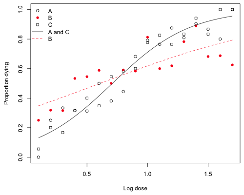
Fig. 1 Dose response models for product B and products A and C together
To find the odds ratios for the effect of dosage we need to exponentiate the slopes that are shown in Table 1.
So for every one unit increase in log dose, the odds of dying increases by a factor of 22.17 for products A and C, but only by a factor of 3.43 for product B.
To obtain a confidence interval for an odds ratio we first calculate the confidence interval for the log odds ratio and then exponentiate the endpoints. To obtain this for product B we need the variance of a sum, coef(out3)[2] + coef(out3)[4]. The method for doing this was explained in lecture 5 and involves extracting the variance-covariance matrix of the parameter estimates and then constructing a quadratic form.
A shortcut method for doing this was also given in lecture 5. We fit the model without the logdose main effect and remove the intercept. When there is a factor in the model, R reports the actual estimates at each level of the factor rather than reporting the estimates of the effects as it normally does.
Using this output the Wald-based confidence intervals are obtained as follows.
The likelihood-based confidence intervals can be obtained by using the confint function on this last model.
The two types of intervals are quite similar.
| Jack Weiss Phone: (919) 962-5930 E-Mail: jack_weiss@unc.edu Address: Curriculum for the Environment and Ecology, Box 3275, University of North Carolina, Chapel Hill, 27599 Copyright © 2012 Last Revised--February 23, 2012 URL: https://sakai.unc.edu/access/content/group/2842013b-58f5-4453-aa8d-3e01bacbfc3d/public/Ecol562_Spring2012/docs/solutions/assign5.htm |