Lecture 9—Monday, January 30, 2012

Topics

• Maximum likelihood estimates
  • Why are MLEs attractive?
  • Some problems with MLEs
  • Maximum likelihood estimation versus ordinary least squares
• Significance testing and maximum likelihood estimation
  • Likelihood ratio tests
  • Wald tests
  • Wald confidence intervals
  • Likelihood-based confidence intervals
• Model selection criteria

R functions and commands demonstrated

• attr can be used to extract attributes from R objects
• logLik extracts the log-likelihood from a model object
• pchisq is the cumulative distribution function of a chi-squared distribution
• qchisq is the quantile function of a chi-squared distribution

Maximum likelihood estimates (MLEs)

We begin by considering some of the more theoretical aspects of maximum likelihood estimation. Because MLEs are calculated from a sample, the value obtained will vary from sample to sample. Hence MLEs have a sampling distribution and we can talk about the characteristics of that distribution and using it as a basis for constructing confidence intervals.

Why are MLEs attractive?

1. They are intuitive. The notion of selecting values for the parameters in order to make the data most probable under a given model is appealing.
2. MLEs have a number of nice statistical properties. Most of these are rather technical.
3. The sampling distribution of MLEs is asymptotically normal with known variance. Thus if the sample is large enough statistical tests can be carried out and confidence intervals constructed by appealing to normality.
4. The log-likelihood has a connection to information theory that yields a method for comparing non-nested models using the AIC statistic.

Some problems with MLEs

1. There are no concrete rules for deciding when a sample is big enough for the assumption of normality to hold. Thus statistical tests carried out using maximum likelihood estimates can be suspect.
2. MLEs can be biased with small samples.

The term bias has a very specific meaning to a statistician. An estimate is unbiased for a parameter θ if the mean of the sampling distribution of is equal to θ. A statistician writes this as , where E is the expectation operator and is defined as "take the mean". An unbiased estimator has a sampling distribution that is centered over the true population value. Fig. 1 shows the sampling distributions of two estimators, and . Estimator is unbiased. The mean of its distribution is equal to the population value θ. The estimator is biased. It's distribution is centered on a value less than θ and hence on average will underestimate the population value θ.

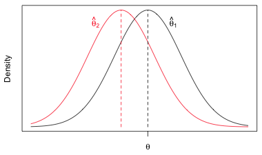
Fig. 1  Bias: estimator is unbiased for θ, while estimator is biased for θ. (R code)

The bias of maximum likelihood estimates, when present, tends to disappear as the sample size increases. Thus MLEs are said to be asymptotically unbiased.

Maximum likelihood estimation versus ordinary least squares

To illustrate the connection between MLE and OLS consider the problem of obtaining maximum likelihood estimates of the parameters of a simple linear regression model in which the response is assumed to be normally distributed. The model in question is the following.

If we have a sample of size n, the likelihood of this model, using R notation, is the following.

and the log-likelihood is

To find the maximum likelihood estimates by hand we could use calculus. Calculus tells us that interior maxima occur at stationary points, i.e., points where all of the partial derivatives of our objective function are zero. Thus we could calculate the partial derivatives of the log-likelihood with respect to the three parameters, set them equal to zero, and try to solve them for the individual parameters.

In doing this for the normal model a number of terms drop out. In the end maximizing the original log-likelihood simplifies to maximizing the following quantity:

This is the negative SSE, the sum of squared errors that is minimized in ordinary least squares. So, maximizing the log-likelihood is the same as maximizing –SSE which is the same as minimizing SSE. The upstart is that in the case of the normal regression model, maximum likelihood estimation and ordinary least squares yield the same solutions for the regression parameters.

Ordinary least squares does not directly yield an estimate for σ, but motivated by the signal plus noise interpretation of ordinary least squares, the mean squared error of the model, MSE, is a natural choice for estimating σ². The formula used is the following.

where p is the number of estimated regression parameters and n is the sample size. For the simple linear regression example we've considering, p = 2, corresponding to the slope and intercept.

In the maximum likelihood approach when we solve the partial derivative equations for σ we obtain a slightly different estimate of σ².

The two estimates differ in their choice of denominator. Because the MLE has a bigger denominator its estimate of σ is slightly smaller. It turns out that the OLS estimate is unbiased (that's why it was chosen) whereas the MLE of σ is biased. On the other hand the MLE of σ is clearly asymptotically unbiased because when n is big, the difference between n and n – p is small and the effect on the estimate will be negligible.

Significance testing and maximum likelihood estimation

In ordinary least squares there are two kinds of statistical tests that are useful in model simplification: the partial F-tests that are returned by the anova function of R and the individual t-tests that appear in the coefficients table produced by the summary function of R. Each of these tests has an equivalent version in the likelihood-based framework. The partial F-tests are replaced by likelihood ratio tests and the individual t-tests are replaced by Wald tests. We consider each of these in turn.

Likelihood ratio tests

Consider the following three Poisson models that were fit last time.

Here z₂, z₃, and z₄ are dummy variables indicating weeks 2, 3, and 4 respectively.

Beginning with the most complex model we should first test whether the interaction terms are necessary thus determining if the coefficient of NAP varied by week. The corresponding hypothesis test is the following.

H₀: β₅ = β₆ = β₇ = 0
H₁: at least one of β₅, β₆, β₇ is not zero

This hypothesis tests whether model mod3p can be reduced to model mod2p. When two nested models are fit by maximum likelihood they can be compared using what's called a likelihood ratio test. The test statistic is the following.

where log L(mod3) and log L(mod2) are the log-likelihoods of mod3 and mod2 respectively. Notice that the larger, more complicated model appears in the numerator. The second equality shown in the above expression follows from a property of logarithms: the logarithm of a quotient is the difference of two logs.

The likelihood ratio statistic has a large sample chi-squared distribution with degrees of freedom given by the difference in the number of parameters in the two models. Put another way the degrees of freedom is the number of parameters we need to eliminate in the larger model to turn it into the smaller model.

where df = #parameters in mod3 – #parameters in mod2

The likelihood ratio test is a one-sided upper-tailed test. We reject the null hypothesis if the LR statistic is too big. We can extract the log-likelihood of a model in R with the logLik function.

The quantities in parentheses that appear after the log-likelihood and are labeled df are the number of parameters that were estimated in each model. The number of estimated parameters, df, is an attribute of the logLik object and can be extracted with the attr function as follows.

The quantities needed for the likelihood ratio test are calculated as follows.

The p-value of the test statistic is . It can be obtained using the pchisq function which calculates P(X ≤ k) where X has a chi-squared distribution.

Because the p-value is small (less than .05) we reject the null hypothesis and conclude that one or more interaction term coefficients are different from zero and hence should be retained. Instead of calculating a p-value we could calculate the critical value of our test using the qchisq function.

Because the observed value of the likelihood ratio statistic, 22.4, exceeds the critical value of 7.81, we reject the null hypothesis.

It is unnecessary to carry out the likelihood ratio test by hand because the anova function of R will do it for us. If we give anova two nested models and specify test='Chisq' it will carry out a likelihood ratio test to see if the more complicated model can be reduced to the simpler model.

Model 1: richness ~ NAP + factor(week)
Model 2: richness ~ NAP * factor(week)
  Resid. Df Resid. Dev Df Deviance  Pr(>Chi)   
1        40     53.466                         
2        37     31.070  3   22.396 5.396e-05 ***
---
Signif. codes:  0 ‘***’ 0.001 ‘**’ 0.01 ‘*’ 0.05 ‘.’ 0.1 ‘ ’ 1

Observe that the test statistic, labeled Deviance, and the p-value, labeled PR(>Chi), are identical to what we calculated above.

Just as with normal models, using the anova function on a single model estimated using maximum likelihood causes R to carry out a sequence of tests. These tests will be likelihood ratio tests if test='Chisq' is also specified.

Model: poisson, link: log

Response: richness

Terms added sequentially (first to last)

                 Df Deviance Resid. Df Resid. Dev  Pr(>Chi)   
NULL                                44    179.753             
NAP               1   66.571        43    113.182 3.376e-16 ***
factor(week)      3   59.716        40     53.466 6.759e-13 ***
NAP:factor(week)  3   22.396        37     31.070 5.396e-05 ***
---
Signif. codes:  0 ‘***’ 0.001 ‘**’ 0.01 ‘*’ 0.05 ‘.’ 0.1 ‘ ’ 1

The column labeled Deviance reports the likelihood ratio statistics for various tests. The three tests carried out are the following.

1. Row 2 labeled NAP compares a model with NAP in it (mod1p) to a model with only an intercept. This is a 1 degree of freedom test (corresponding to the single coefficient of NAP) and tests the null hypothesis that the coefficient of NAP is equal to zero. The small reported p-value indicates that we should reject the null hypothesis.
2. Row 3 labeled factor(week) compares a model with both NAP and factor(week) in it (mod2p) to a model with only NAP (mod1p). This is a 3 degrees of freedom test because there are three dummy variables for week. It tests the null hypothesis that the coefficients of all three dummy variables are zero. The small p-value indicates that we should reject this null hypothesis.
3. Row 4 labeled NAP:factor(week) compares the interaction model (mod3p) to the additive model (mod2p). This is the same test that we carried out above with anova(mod2p, mod3p, test='Chisq').

Wald tests

Wald tests are reported in the coefficients table that is produced when the summary function is applied to a glm model. Like the t-tests shown in the summary output of an lm object, Wald tests are variables-added last tests, thus not all of the tests reported in the coefficients table will necessarily make sense. When there are categorical variables in a model the Wald tests are useful for determining which of the groups are different.

From the output we see that coefficient of NAP is negative but not significantly different from zero in week 1 (p = 0118). The three interaction terms then test if the coefficients of NAP in weeks 2, 3, and 4 are different from the value in week 1. From the output the coefficient of NAP in week 4 is certainly different from what it is in week 1. For weeks 2 and 3 the results are less clear: the slope in week 3 is significantly different (p = 0.026) but the slope in week 2 just misses being significantly different (p = 0.053). The estimates of the differences are all negative indicating that the coefficients of NAP in weeks 2, 3, and 4 are even more negative than they are in week 1.

Because Wald tests and likelihood ratio tests make different assumptions about the likelihood, the two tests need not agree even when they are testing the same hypothesis. Both are large-sample tests but the general recommendation is that when sample sizes are small, the results from likelihood ratio tests tend to be more trustworthy than the results from Wald tests.

Wald-based Confidence intervals

The maximum likelihood estimates of regression parameters are asymptotically normal, thus we can construct normal-based Wald confidence intervals for the parameters using the estimates and standard errors reported in the summary table output. The summary coefficient table is just a matrix so we can access its entries by row and column number. For example, the calculation below obtains the 95% confidence interval for the coefficient of NAP.

If we leave off the row numbers in the above calculation we can obtain 95% confidence intervals for all of the estimates in the summary table.

Likelihood-based confidence intervals

Confidence intervals can also be constructed based on the likelihood ratio test. These are called profile likelihood confidence intervals and are calculated when the confint function is applied to a glm model object.

In this case the results we obtain are very close to the Wald-based results.

Model selection criteria

Significance testing can be used to choose between models but only when those models are nested. What about comparing models that are not nested or comparing models that use different probability models? For instance suppose we fit the same model to data but in one case we assume the response has a Poisson distribution and in the other case we assume it is normally distributed.

For count data if we interpret the normal densities in the likelihood for the normal model as being midpoint approximations of the probabilities of the individual counts, then we can compare these two models directly using log-likelihood (see lecture 8). The model with the larger log-likelihood is the one that makes our data more probable.

Based on the reported log-likelihoods the data are more probable (greater log-likelihood) under the normal model than under the Poisson model.

In truth this isn't a fair comparison. The normal model uses three parameters: β₀, β₁, and σ² whereas the Poisson model uses just two. It is easier to fit data when one has more parameters at one's disposal. John von Neumann is famously reported to have said, "With four parameters I can fit an elephant, but with five I can make him wiggle his trunk." The log-likelihood can never decrease as one adds additional parameters to a given probability model. At worse, it will remain the same. So perhaps a better strategy is to penalize a model that fits better but does so at the cost of estimating more parameters.

There have been many ad hoc methods proposed to penalize models that have become too complex. In ordinary linear regression two such criteria are adjusted R² and Mallow's C_p.

adjusted R²:

Mallow's C_p:

Here n is the sample size, p is the number of parameters in the model, s² = MSE for the full model (i.e., is the model containing all k explanatory variables of interest), SSE_p is the residual sum of squares for the subset model containing p parameters including the intercept, and R² is the ordinary R² statistic (coefficient of determination). Both adjusted R² and Mallow's C_p end up penalizing those models that include parameters that contribute very little explanatory power to the model.

Penalized measures also exist for likelihood-based models where they are referred to as information-theoretic criteria. Three popular ones are AIC, AIC_c, and BIC.

Here log L is the log-likelihood of the model, k is the number of parameters that were estimated, and n is the sample size. AIC_c is a small sample correction to AIC and is recommended when the ratio of n to k is less than 40, i.e., . In other cases the difference between AIC and AIC_c is negligible.

These three statistics differ in the way that they penalize complexity. AIC and its small sample alternative AIC_c stand out because they are more than ad hoc corrections to the log-likelihood. They also have a strong theoretical basis in information theory. We'll explore this theoretical basis next time.

Course Home Page