
Fig. 1 Kaplan-Meier estimate of the seedling survivor function
The data are taken from a Master's thesis in which the goal is to determine the habitat requirements of the rare plant species Tephrosia angustissima with the goal of eventually reintroducing it into portions of its historical range where it has been extirpated. Additional details of the study can be found at the Fairchild Tropical Botanic Garden web page. Greenhouse-raised parents were planted in three distinct habitats. All of their progeny were marked and their survival history was recorded. The first few observations from the data set are shown below. Each row corresponds to an individual seedling.
This is an example of a staggered entry data set. A seedling's survival history began when it was first observed in the field. To estimate the survivor function all individuals must have the same start time. Thus we need to create an age variable from the staggered entry dates.
The variables Start.Date and Last.Observed were treated as character data by R and converted to factors by the read.csv function when the data were read in. To calculate a seedling's age at death (or censor time), we need to get R to treat these values as actual dates. The as.Date function of base R can be used to convert character data into date data. To use it we enter the character representation of the date as the first argument and a string that identifies the manner in which the date is formatted as the second argument. The string consists of conversion specifications that are introduced by the % character usually followed by a single letter. A full list of conversion specifications are given in the help screen of the strptime function.
The dates in the seedlings file are presented in the order month, day, followed by a four-digit year all separated by forward slashes. The format string we need to use that identifies this arrangement is "%m/%d/%Y". Then to obtain the age of a seedling we subtract the start date from the last observed date.
Observe that the print out for the Age variable just created includes some unusual formatting. To see what kind of object we've created we can use the class function.
The survival functions we'll be using can't work with objects that have date classes, so we need to convert these date differences into numbers with the as.numeric function. Here's the complete command after this additional modification.
The package survival contains functions for carrying out survival analysis. The first step in any analysis is to use the Surv function to create a survival object. For right censored data we need to specify two arguments: the variable that records the age at the event time followed by the variable that identifies the nature of the event (failure or censored). The survfit function then uses the Surv object as the response variable in a formula expression to produce the Kaplan-Meier estimate of the survivor function. The standard approach is to create the Surv object and estimate the survivor function in a single expression.
The component $surv of the survfit object is the Kaplan-Meier estimate while $upper and $lower components are the upper and lower 95% confidence limits. If we use the plot function on a survfit object, we get the a plot of the estimated survivor function along with a 95% confidence band.
|
|---|
Fig. 1 Kaplan-Meier estimate of the seedling survivor function |
To obtain separate estimates of the survivor function by habitat we enter the habitat variable as a factor on the right side of the survfit formula.
 |
|---|
Fig. 2 Kaplan-Meier estimate of the seedling survivor function separately by habitat |
The tick-marks shown on the individual curves represent ages at which individuals were censored.
It is possible to add confidence bands to each curve by specifying conf.int=T as an argument to plot (actually the plot.survfit method). Unfortunately the confidence bands that appear are not distinguished from the estimate (using different line types or colors) and the display can get confusing. To superimpose the 95% confidence bands on this graph each with their own line types we need to add them ourselves. To accomplish this we have to understand how the estimates and confidence limits are organized in the survfit object that was created. When a factor variable is included on the right side of the formula expression, a new component called $strata is generated in the survfit object. It tells us the number of observations in the individual strata and the order they occur in the returned estimates.
We can use this variable to create an indicator variable that identifies the stratum from which each estimate comes.
Using this variable we can variously select the estimates for habitats 1, 2, and 3 and add the confidence bands to the above plot with the lines function.
From the plot we see that while habitats 1 and 2 exhibit different survivorship patterns initially that then converge, individuals in habitat 3 persist longer than individuals in the other two habitats at every age.
 |
|---|
Fig. 3 Kaplan-Meier estimates of the seedling survivor function given separately by habitat with 95% confidence bands |
The survdiff function carries out the log-rank test to test for differences in the survivor function between groups. Its syntax is identical to that of the survfit function.
N Observed Expected (O-E)^2/E (O-E)^2/V
factor(HabitCode)=1 1119 1116 934 35.58 110.3
factor(HabitCode)=2 260 258 307 7.79 11.9
factor(HabitCode)=3 233 212 345 51.50 86.5
Chisq= 123 on 2 degrees of freedom, p= 0
The survdiff function has an argument rho that allows one to weight observations in the survival history differently. The default value is rho=0 for which the weights are all equal to one. If we set rho=1 we obtain the Gehan-Wilcoxon test that weights early differences in survivorship more heavily than differences at later survival times. The weights in this case are the number of individuals that are still at risk at each event time.
N Observed Expected (O-E)^2/E (O-E)^2/V
factor(HabitCode)=1 1119 660.3 558 18.9 88.7
factor(HabitCode)=2 260 118.4 164 12.5 26.2
factor(HabitCode)=3 233 95.7 153 21.5 45.8
Chisq= 90.4 on 2 degrees of freedom, p= 0
The conclusions are the same for both versions of the test but notice that the value of the test statistic is much larger for the ordinary log-rank test indicating that late survival time differences are larger than early survival time differences. This is also clear from Fig. 3.
The coxph function fits the Cox proportional hazards regression model. Its syntax is identical to that of other regression functions in R except that it does require the response to be a survival object created by the Surv function.
n= 1612
coef exp(coef) se(coef) z Pr(>|z|)
factor(HabitCode)2 -0.37936 0.68430 0.06932 -5.473 4.43e-08 ***
factor(HabitCode)3 -0.76908 0.46344 0.07719 -9.963 < 2e-16 ***
---
Signif. codes: 0 ‘***’ 0.001 ‘**’ 0.01 ‘*’ 0.05 ‘.’ 0.1 ‘ ’ 1
exp(coef) exp(-coef) lower .95 upper .95
factor(HabitCode)2 0.6843 1.461 0.5974 0.7839
factor(HabitCode)3 0.4634 2.158 0.3984 0.5391
Rsquare= 0.075 (max possible= 1 )
Likelihood ratio test= 125.9 on 2 df, p=0
Wald test = 113.3 on 2 df, p=0
Score (logrank) test = 117.1 on 2 df, p=0
In Cox regression we model the log hazard so the fact that the coefficient estimates are negative and statistically significant tells us that plants in habitats 2 and 3 experience a significantly lower hazard than do plants in habitat 1, the reference group. The exponentiated coefficients shown in the output are the hazard ratios. The hazard ratios labeled exp(-coef) have switched things around so that habitats 2 and 3 are the reference groups, and habitat 1 is the test group. Using these we see that the hazard of dying at any instant is 1.46 times greater in habitat 1 than in habitat 2, and 2.16 times greater in habitat 1 than in habitat 3.
The coxph object that was created has a method for the anova function from which we can obtain an overall test of the construct HabitCode. With just one predictor this is identical to the likelihood ratio test reported in the summary table.
loglik Chisq Df Pr(>|Chi|)
NULL -10229
factor(HabitCode) -10166 125.86 2 < 2.2e-16 ***
---
Signif. codes: 0 ‘***’ 0.001 ‘**’ 0.01 ‘*’ 0.05 ‘.’ 0.1 ‘ ’ 1
Although the baseline hazard is not estimated in a Cox model, it is still possible to obtain an estimate of the survivor function by applying the survfit function to a coxph object. It returns an estimate that is similar to the Kaplan-Meier estimate calculated from raw data. According to the help screen for survfit, "When the parent data is a Cox model, there is an extra term in the variance of the curve, due to the variance of the coefficients and hence variance in the computed weights." For Cox models it is necessary to specify values for the variables in the model using the newdata= argument. I obtain these estimates for each habitat type by specifying different values for the HabitCode variable, plot the results, and superimpose the ordinary Kaplan-Meier estimates for comparison.
 |
|---|
Fig. 4 Kaplan-Meier and Cox estimates of the seedling survivor functions separately by habitat |
So far the Cox model hasn't given us anything more than we already obtained with the ordinary Kaplan-Meier estimate and the log-rank test. The real reason for fitting a Cox model is to include additional predictors for statistical control in order to obtain more realistic estimates of the standard errors. Recall that these data are heterogeneous—some come seedlings from the same parent and other seedlings come from different parents. Seedlings from the same parent are likely to be close spatially and more similar genetically. Mixed effects models in survival analysis are called frailty models and while they are available in R they are sometimes difficult to fit. A GEE alternative to frailty models calculates robust sandwich estimates of the variances of the parameter estimates for the Wald tests (univariate and multivariate) that are reported in the output. We can obtain robust sandwich estimates with the cluster function by identifying Parent as the source of the heterogeneity and then including this as a term in the model.
n= 1612
coef exp(coef) se(coef) robust se z Pr(>|z|)
factor(HabitCode)2 -0.37936 0.68430 0.06932 0.12236 -3.100 0.00193 **
factor(HabitCode)3 -0.76908 0.46344 0.07719 0.14345 -5.361 8.26e-08 ***
---
Signif. codes: 0 ‘***’ 0.001 ‘**’ 0.01 ‘*’ 0.05 ‘.’ 0.1 ‘ ’ 1
exp(coef) exp(-coef) lower .95 upper .95
factor(HabitCode)2 0.6843 1.461 0.5384 0.8697
factor(HabitCode)3 0.4634 2.158 0.3499 0.6139
Rsquare= 0.075 (max possible= 1 )
Likelihood ratio test= 125.9 on 2 df, p=0
Wald test = 29.86 on 2 df, p=3.281e-07
Score (logrank) test = 117.1 on 2 df, p=0, Robust = 22.14 p=1.558e-05
(Note: the likelihood ratio and score tests assume independence of
observations within a cluster, the Wald and robust score tests do not).
The new results obtained by including the cluster function are highlighted in the above output. Specifying Parent as a source of clustering has changed the reported p-values and confidence intervals, but it has not altered any of our conclusions. Habitat is still seen to have a significant effect on survival.
Another reason for fitting a Cox model is to include control variables in the model, variables that might be confounders of the effect of interest. This is not a primary issue with these data because most of the available explanatory variables are just surrogates for habitat. One variable that may be an exception to this is parentlight, which was measured at the beginning of study and was an attempt to account for the different microhabitats experienced by individual seedlings.
Call:
coxph(formula = Surv(Age, SdlgCensor) ~ factor(HabitCode) + cluster(Parent) +
parentlight, data = seedlings)
n= 1535, number of events= 1509
(77 observations deleted due to missingness)
coef exp(coef) se(coef) robust se z Pr(>|z|)
factor(HabitCode)2 -0.25088 0.77812 0.07285 0.13276 -1.89 0.059 .
factor(HabitCode)3 -0.82102 0.43999 0.07914 0.13630 -6.02 1.7e-09 ***
parentlight 0.00464 1.00465 0.00095 0.00226 2.05 0.040 *
---
Signif. codes: 0 ‘***’ 0.001 ‘**’ 0.01 ‘*’ 0.05 ‘.’ 0.1 ‘ ’ 1
exp(coef) exp(-coef) lower .95 upper .95
factor(HabitCode)2 0.778 1.285 0.600 1.009
factor(HabitCode)3 0.440 2.273 0.337 0.575
parentlight 1.005 0.995 1.000 1.009
Concordance= 0.588 (se = 0.01 )
Rsquare= 0.086 (max possible= 1 )
Likelihood ratio test= 138 on 3 df, p=0
Wald test = 38.6 on 3 df, p=2.09e-08
Score (logrank) test = 132 on 3 df, p=0, Robust = 21.2 p=9.59e-05
(Note: the likelihood ratio and score tests assume independence of
observations within a cluster, the Wald and robust score tests do not).
The Wald test with the robust standard errors finds this predictor to be statistically significant.
For categorical predictors the proportional hazards assumption can be assessed by plotting log(–log(S(t))) against time separately for the different habitat categories. If the proportional hazards assumption holds the curves should be parallel. Here S(t) is the KM estimate of the survivor function for the different categories. I examine whether the proportional hazards assumption is satisfied for the individual habitats. Although the KM estimates were obtained earlier I repeat the calculations below.
 |
|---|
Fig. 5 Graphical assessment of the proportional hazards assumption for the predictor habitat |
While the curves for habitat 1 and 3 are parallel, the curve for habitat 2 is clearly not parallel to the other two suggesting that the proportional hazards assumption for this variable may be incorrect.
Suppose subject i has an event at time tj. Then the Schoenfeld residual for this subject for a given predictor is the observed value of that predictor minus a weighted average of the predictor values for the other subjects still at risk at time tj. The weights used are each subject’s estimated hazard. The idea behind the statistical test is that if the proportional hazards assumption holds for a particular covariate then the Schoenfeld residuals for that covariate will not be related to survival time.
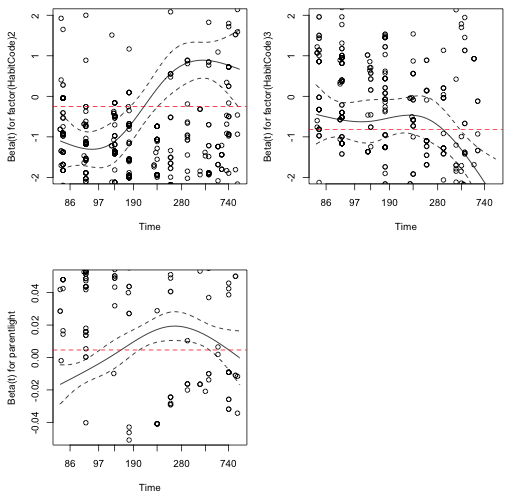
The cox.zph function in the survival package uses this approach to assess the proportional hazards assumption. When we plot the object created by cox.zph we get estimates of a time-dependent coefficient for each predictor in the mode, labeled beta(t) in the plot. If the proportional hazards assumption is correct, beta(t) will be a horizontal line at the value returned by coxph for this parameter. The printout from the function call provides a test that slope of this line is 0 for each regressor.
The displayed p-value tests whether the individual regression coefficients are constant over time. According to the test results above we should reject this for all of the regressors in the model. Of course the clustering of observations around parents may be inflating the magnitude of these relationships so perhaps we should not take the p-values too literally.
If we plot the cox.zph object we get a graphical display of how the different regression coefficients estimated change over time. The ylim argument is used to zoom in on the displayed pattern.
 |
|---|
Fig. 6 A graphical assessment of the proportional hazards assumption: a plot of the individual estimated regression coefficients against time with the estimate from the Cox model superimposed. |
The coefficient estimates from coxph for the habitat effect regressors are negative, while the estimate for the parent light variable is positive. In Fig. 6 it appears that the first habitat dummy regressor coefficient and the parentlight coefficient start negative and then become positive over time. More importantly we see that the coefficient estimates from the Cox model (the horizontal lines in the graphs) do not lie entirely within the displayed confidence bounds at all the survival times. (The habitat 3 coefficient comes closest but exits the confidence bands for long survival times.) Based on Fig. 6 the constant estimates returned by the Cox model for each parameter are implausible and would be rejected at many of the survival times.
Option 1. In Fig. 6 the variable parentlight appears to have a quadratic relationship with time. Perhaps it also has a quadratic relationship with the hazard. Such a relationship is biologically motivated. One might expect that there would be an intermediate optimal light level for survival rather than a strictly linear relationship.
The test for time-varying coefficients is no longer significant for parentlight. On the other hand the quadratic coefficient is not statistically significant when we use robust standard errors, although it is statistically significant at α = .05 if we use the naive standard error.
Option 2. For categorical variables we have the option of stratifying by levels of the categorical variable. In a Cox model this means assuming different baseline hazards for each level but still using all the data in estimating the remaining regression coefficients. To carry this out with coxph we use the strata function rather than the factor function on the variable HabitCode.
The down side to this approach is that no estimates are returned for the stratifying variable, hence in this case there is no way to assess statistically whether survivorship differs by habitat.
Parametric survival models are fit in R with the survreg function of the survival package. I focus here exclusively on Weibull models. Depending on the parameterization, a Weibull model can be viewed as either a proportional hazards (PH) model or an accelerated failure time (AFT) model. R fits the accelerated failure time parameterization.
Scale= 0.688
Weibull distribution
Loglik(model)= -10345.5 Loglik(intercept only)= -10429.7
Chisq= 168.36 on 2 degrees of freedom, p= 0
Number of Newton-Raphson Iterations: 5
n= 1612
As is explained in lecture 28, in the AFT parameterization of the Weibull distribution we model what is usually called the log scale parameter, log λ, with a linear predictor. This is essentially equivalent to modeling log survival time. Confusingly, another parameter in the survreg output is labeled log(scale). This reversed notation is peculiar to survreg. What survreg calls the scale parameter is in fact the reciprocal of what is usually called the shape parameter. Based on the positive coefficient estimates shown in the above output for HabitCode we can conclude that plants in habitats 2 and 3 live significantly longer (their survival times are more stretched out) than those in habitat 1.
Although not needed here it is possible to adjust the default optimization settings with the control argument coupled with the survreg.control function. For instance, the following settings increase the maximum number of iterations from the default value of 30 to 100.
There are a number of ways of displaying the results from the Weibull analysis. We can use the predict function on the survreg model object and request percentile estimates for designated percentiles and plot the results. For this we need to use the p= argument to specify a list of the quantile points of the cumulative distribution function. In the code below I generate a sequence of equally spaced percentiles but stop at the 99th percentile because the 100th percentile is at infinity. I specify type="quantile" to obtain the quantile predictions. Using the matplot function to generate the plot is a shortcut; it plots the estimate and 95% confidence bands all at the same time with a single function call.
 |
|---|
Fig. 7 Estimate of the Weibull survivor function with 95% confidence bands |
We can perhaps obtain more accurate coverage by constructing the confidence intervals on the log scale and then exponentiating the result. To obtain an estimate of the quantiles of the survivor function on the scale of the linear predictor we need to specify type='uquantile'. After calculating the confidence bounds for the log quantiles we then need to exponentiate the result.
For these data the plot that results is essentially identical to Fig. 7 and is not shown.
The labeling of the Weibull parameters in the survreg function even differs from that used by the Weibull function in base R. As was mentioned above the linear predictor is the estimate of what is usually called log scale, i.e. log λ, and what survreg calls the scale parameter is in fact the reciprocal of the Weibull shape parameter used in the base R Weibull functions. With those identifications understood, plotting the Weibull survivor function becomes straight-forward. Just use the pweibull function with the argument lower.tail=FALSE, or equivalently, plot instead 1–pweibull.
 |
|---|
Fig. 8 Weibull survivor functions for individual habitats |
Fig. 8 compares the estimate of the survivor function in habitat 1 using the Cox model with the estimated obtained using Weibull regression. As the plot demonstrates the two estimates coincide fairly closely. The Weibull model estimate resembles a smoothed version of the Cox model estimate.
 |
|---|
Fig. 9 Comparison of the Weibull and Cox estimates of the survivor function for habitat 1 |
In a similar fashion we can obtain estimates of the Weibull densities and the Weibull hazard functions in the three habitats.
 |
 |
|---|---|
Fig. 10 Estimated Weibull density and hazard functions for each habitat |
|
For a model with only categorical variables a graphical test of the Weibull model is to plot log(-log(S(t))) versus log t separately for each category. Here S(t) is the usual Kaplan-Meier estimate. The key result derived from this plot is that straight but not necessarily parallel lines support the Weibull assumption while parallel curves support the proportional hazards (PH) assumption.
 |
|---|
Fig. 11 Graphical assessment of the Weibull assumption |
The following is a summary of the possible results and recommended actions for a plot of log[−log S(t)] against log t as taken from Kleinbaum & Klein (2005), p. 274.
The lines shown in Fig. 11 are clearly not parallel but, except for a couple of early values in habitat 3, they may not be that far from being straight. According to the recommendations given above we should try a Weibull model in which we let the shape parameter vary by habitat. In the survreg function we can request different shape parameters by using the strata function. Interestingly survreg allows us to vary both the shape and scale parameters by habitat. We do this by letting habitat appear both as a predictor and as an argument of the strata function.
When we compare the three Weibull models using AIC we find that a model in which both the scale and shape parameters vary by habitat fits best. The summary of the best model is shown below. In the summary table the last three coefficient estimates are what R calls the log(scale) parameters (but really correspond to the shape parameters in the manner explained above).
Scale:
HabitCode=1 HabitCode=2 HabitCode=3
0.678 0.631 0.821
Weibull distribution
Loglik(model)= -10337.9 Loglik(intercept only)= -10384.8
Chisq= 93.68 on 2 degrees of freedom, p= 0
Number of Newton-Raphson Iterations: 5
n= 1612
The seedlings were examined episodically every few months rather than continuously. Thus it is perhaps better to treat all of the observations as interval censored. The survreg function does support interval censoring. The variables left.bound and right.bound in the seedlings data frame record the last time a seedling was seen alive and the very next observation period respectively (at which time it was not found). To let R know that interval censoring is desired, the type="interval2" argument is used in the Surv function. One peculiar aspect of using interval-censored data in a Weibull model is that observations whose censor intervals are of the form (0, x), where x is some value and hence are really left-censored, must instead be recorded as (NA, x) because 0 is not a legal value in the Weibull distribution. Similarly, truly right-censored observations must be recorded with the interval (x, NA). These adjustments have already been made to the variables left.bound and right.bound. The syntax for fitting the model with survreg is shown below.
Scale= 0.804
Weibull distribution
Loglik(model)= -2727 Loglik(intercept only)= -2773.7
Chisq= 93.5 on 2 degrees of freedom, p= 0
Number of Newton-Raphson Iterations: 4
n= 1612
The basic conclusions about the effect of habitat on survival do not change when we treat the data as interval censored.
| Jack Weiss Phone: (919) 962-5930 E-Mail: jack_weiss@unc.edu Address: Curriculum for the Environment and Ecology, Box 3275, University of North Carolina, Chapel Hill, 27599 Copyright © 2012 Last Revised--April 5, 2012 URL: https://sakai.unc.edu/access/content/group/2842013b-58f5-4453-aa8d-3e01bacbfc3d/public/Ecol562_Spring2012/docs/lectures/lecture29.htm |